1 Data Types
Data scientists work with different kinds of data.
We have already seen two different types in the previous chapters: numerical data (e.g., 14 or 1.5 ) and text data (e.g., "you found yourself in a wide, low, straggling entry with old-fashioned wainscots").
These different representations of data are often referred to as data types.
In this chapter we will learn about four fundamental data types in R and how the tidyverse can be used for working with them.
They are:
- a whole number, which we call the integer type
- a real number, which we call the double type
- a truth value representing TRUE or FALSE, which R calls the logical type. These are also often called the boolean type, especially in other programming languages.
- a character sequence, which R calls the character type. These are commonly referred to as the string type.
We will also study two important structures for storing data known as the vector and the list.
1.1 Integers and Doubles
In this section, we turn to our first two principal data types: the integer and the double.
1.1.1 A primer in computer architecture
The vacuum tubes we mentioned earlier as one of the principal ideas in the early modern computers had the role of regulating flow of electricity. The architects of the machines used two conditions, the existence of current and the non-existence of current, for information coding.
We used the word bit to present the dichotomy, 1 for having the current and 0 for not having the current. All the computer models that followed used the principle.
An integer type consists of some fixed number of (for example, 32) bits. In its simplest representation, one of the bits is used to represent the sign (1 for negative numbers and 0 for non-negative numbers) and the rest are to represent the absolute value of the number with the power-of-2 denominations.
The power-of-2 denominations consist of the powers of 2 in increasing order starting from the 0-th power (which is equal to 0): \(2^0 = 1, 2^1 = 2, 2^2 = 4, 2^3 = 8, 2^4 = 16, \ldots\).
We call this the binary representation as opposed to the decimal representation as we write numbers in our daily life.
For example,
\[ 0 \cdots 0 1 1 1 0 1 \] in the representation is to represent by reading the bits from right to left,
\[ 1 \cdot 2^0 + 0 \cdot 2^1 + 1 \cdot 2^2 + 1 \cdot 2^3 + 1 \cdot 2^4 \]
which is equal to \(1 + 4 + 8 + 16 = 29\).
This implies that there is a limit to how large a positive whole number or how small a negative whole number R can accurately represent. If a number should go out of the range of accurately-presentable whole numbers, R switches to a double number using some approximation.
To represent a double number, computers split the number of bits it can use to three parts: the sign (1 bit), the significand, and the exponent. How R uses the significand and exponents in representing a real number is beyond the scope of this text.
\[ (\mathrm{sign}) ~(\mathrm{number~significand~represents}) \cdot (\mathrm{base})^{\mathrm{number~exponent~represents}} \]
The representation in the significand part uses the inverse powers of 2: 1/2, 1/4, 1/8, \(\ldots\), down to a certain value \(1/2^m\), where \(m\) is the length of the significand part.
By combining these fractional quantities, we can obtain an approximation for a number between 1 and 2. Like integer, the double type thus has a range of numbers it can record an approximation.
If you are interested in learning more about digital representations of numbers, sign up for a course in computer organization and architecture!
1.1.2 Specifying integers and doubles in R
Our brief dive into how integers and doubles are represented boils down to two basic ideas:
- Integers are called
integervalues in R. They can only represent whole numbers (e.g., positive, negative, or zero). - Real numbers are called
doublevalues in R. They can represent whole numbers and fractions but there are limitations by how well it approximates some values.
Here are some examples of double values.
1.2## [1] 1.2
3.0## [1] 3
1.5 + 2.2## [1] 3.7We can confirm these are doubles using the typeof function.
typeof(3.0)## [1] "double"However, for numbers without a decimal point, i.e. integers, R will still treat them as double.
3 # here is a value that looks like an integer## [1] 3
typeof(3) # ..but is actually a double!## [1] "double"Hence, to create an integer, we must specify this explicitly by placing an L directly after the number.
Here are some examples.
# Some integer values
2L
## [1] 2
1L + 3L## [1] 4
-123456789L## [1] -123456789We can confirm these are integers using the typeof function.
typeof(-123456789L)## [1] "integer"Check out what happens when we try placing an L after a decimal value!
3.2L## [1] 3.2When a mathematical expression contains a double and an integer, the result is always a double.
The third expression 4L + 1 adds an integer 4 and a double together and so is double.
In the fourth one, 1 is also an integer, and so the result is an integer.
3.5 + 1.2## [1] 4.7
3L + 1.3## [1] 4.3
4L + 1## [1] 5
4L + 1L## [1] 5We can confirm the types using typeof().
typeof(3.5 + 1.2)## [1] "double"
typeof(3L + 1.3)## [1] "double"
typeof(4L + 1)## [1] "double"
typeof(4L + 1L)## [1] "integer"1.1.3 Finding the size limit
How big numbers (or negative with big absolute value) can a double represent?
To specify a double number with a large absolute value, we can use the e expression.
If you type a literal that goes beyond the range, R gives you Inf or -Inf to mean that the number is out of range.
Let’s start with e1000.
-1.0e1000## [1] -Inf
1.0e1000## [1] InfSo, using whether the result is Inf or not, we can explore around where between the boundary from the presentable numbers and the non-presentable numbers are:
1.0e500## [1] Inf
1.0e400## [1] Inf
1.0e300## [1] 1e+300
1.0e310## [1] Inf
1.0e305## [1] 1e+305
1.0e306## [1] 1e+306
1.0e307## [1] 1e+307
1.5e308## [1] 1.5e+308
1.6e308## [1] 1.6e+308
1.7e308## [1] 1.7e+308
1.8e308## [1] Inf
1.790e308## [1] 1.79e+308So, around 1.79e308 is the limit.
The quantity is large enough so as to accommodate the computation we will do in this text.
How about integers?
We can do the same exploration, this time appending the character L at the end of each number literal.
We leave this as an exercise for the reader.
Keep in mind that if you supply an integer that is too big, R will present a warning that the value must be converted to a double.
1.2 Strings
A string is a sequence of characters, which takes its place as our third principal data type. Formally, R calls such sequences character vectors, where the word “vector” should seem like gibberish jargon at this point. In this section, we examine the string type.
1.2.1 Prerequisite
There is a variety of operations that are available in base R for manipulating strings. A part of the tidyverse super-library is the stringr library. We will use a few functions from stringr here, so let us load this package.
1.2.2 Strings in R
We use a matching pair of double quotations or a matching pair of single quotation marks (a matching pair of apostrophes) to mark the start and the end of the character sequence we specify as its contents. An advantage of using the double quotation marks is that single quotation marks can appear in the character sequence.
Here are some examples of strings.
"This is my first string."## [1] "This is my first string."
"We love R!"## [1] "We love R!"
'"Data Science" is a lot of fun :-)'## [1] "\"Data Science\" is a lot of fun :-)"Notice that the R substituted the single quotation marks we used for the last literal with double quotation marks. We can inspect these types as well.
typeof("We love R!")## [1] "character"1.2.3 Conversions to and from numbers
First of all, characters are not compatible with numbers. You cannot apply mathematical operations to strings even if their character contents are interpret-able as numbers.
In other words, "4786" is not the number 4786, but a character sequence with the four characters, "4", "7", "8", and "6".
Knowing that the string can mean the number, we can generate an integer representing the number using the function as.integer.
as.integer("4786")## [1] 4786The as functions are useful also when you want to interpret a string as a double and when you want to interpret a number as a string.
The functions as.double and as.character convert a string to a double number and a number to a string, respectively.
as.double("3.14")## [1] 3.14
as.double("456")## [1] 456
as.character(3.14159265)## [1] "3.14159265"
as.character(-465)## [1] "-465"1.2.4 Length of strings
If you know the contents of the string, you can count the characters in the sequence to obtain its length.
However, if you do not know or if the string is very long, you can rely on R to do the counting for you using str_length from the stringr package.
str_length("310A Ungar, 1365 Memorial Drive, Coral Gables, Florida")## [1] 541.2.5 Substrings
A string is a sequence of characters. Each character composing a string receives a unique position. Let us consider the following string.
my_string <- "song"The positioning starts from the left end of the sequence.
- The first position has value 1.
- The four characters of the string,
"s","o","n", and"g", have positions 1, 2, 3, and 4, respectively. - You can specify a string and two positions and obtain a new string consisting of the characters between the two positions.
For example, the substring from position 2 to position 3 of the string “song” is “on”. We can use the function str_sub from stringr to retrieve substrings.
str_sub("song", 2, 3)## [1] "on"The syntax is str_sub(some_string, start, end) where some_string from which we will build a substring, start is the starting position, and end is the ending position.
You can omit the ending position if it is the last position of the string.
str_sub("song", 2)## [1] "ong"You can also retrieve substrings by searching from the right. If the starting number is less than -1, R looks at the index starting from the right. For instance, the following extracts the substring from the third-to-last to last position.
str_sub("song", -3, -1)## [1] "ong"If the ending position is smaller than the starting position, the substring is the empty.
str_sub("song", 2, 0)## [1] ""1.2.6 String concatenation
We may want to combine multiple strings into a single string. We call such action concatenation.
Let us consider three strings.
str1 <- "data"
str2 <- "science"
str3 <- "rocks"
There are two types of concatenation. One type connects strings with no gap, the other connects strings with on white space inserted in between. We can perform these actions using the str_c function from stringr.
Below, we think of concatenating three strings "data", "science", and "rocks" with the two functions individually.
str_c(str1, str2, str3)## [1] "datasciencerocks"
str_c(str1, str2, str3, sep = " ")## [1] "data science rocks"In the second, we provide a whitespace character " " to the argument sep. The effect obtained is that each individual word is separated by a space.
1.3 Logical Data
As we stated before, boolean is the data type for logical values, true and false. TRUE is the value representing true and FALSE is the one representing false. When you use a number where R is expecting to see a boolean, it interprets 0 as FALSE and any non-zero as TRUE.
Here are the two values.
TRUE## [1] TRUE
FALSE## [1] FALSE1.3.1 Comparisons
While we can specify a boolean value with a boolean literal, we can use comparisons to generate boolean values. In the case of numbers, we can compare the values of two mathematical expressions. Here is an example.
1 + 4 > 7 - 4## [1] TRUEThis asks if the value of 1 + 4 is strictly greater than the value of 7 - 4. The former is 5 and the latter is 3, and so the answer to the comparison is in the affirmative. Therefore, the value of the comparison expression is TRUE.
They represent “is equal to”, “is not equal to”, “is greater than”, “is greater than or equal to”, “is smaller”, and “is smaller than or equal to”.
There are six possible types of comparisons. We will define these in the following table using an example with the numbers 6 and 3. Before looking, can you try to guess them all? Compare your guesses against the table.
| Operator | Meaning | True example | False Example |
|---|---|---|---|
| < | Smaller than | 3 < 6 | 6 < 3 |
| > | Greater than | 6 > 3 | 3 > 3 |
| <= | Smaller than or equal to | 3 <= 3 | 6 <= 3 |
| >= | Greater than or equal to | 6 >= 6 | 3 >= 6 |
| == | Equal to | 3 == 3 | 6 == 3 |
| != | Not equal to | 6 != 3 | 3 != 3 |
An expression can chain together multiple comparisons with the AND operator &, and they all must hold in order for the whole expression to be True.
For example, we can express that 1+1 is between 1 and 3 using the following expression.
1 < (1 + 1) & (1 + 1) < 3## [1] TRUEYou may recall the functions max and min for obtaining the maximum and the minimum from a group of numbers, respectively.
One thing to remember is that the minimum is greater than or equal to the average, and the maximum is greater than or equal to the average.
The equality holds when the two numbers in the group are all identical.
Let us set some numbers to variables x and y and see what the maximum and the minimum functions produce.
x <- 12
y <- 5
min(x, y) <= (x + y)/2
## [1] TRUE
max(x, y) >= (x + y)/2## [1] TRUEHow about the equality?
Assuming that we have executed the previous section of the code, we can reuse x and y in the following computation.
x <- 17
y <- 17
min(x, y) == (x + y)/2
## [1] TRUE
max(x, y) == (x + y)/2## [1] TRUE1.3.2 Boolean operations
There are three fundamental boolean operations.
They are negation, disjunction, and conjunction.
Negation flips the value of a boolean.
Disjunction tests if at least one of boolean values appearing on a list is true and conjunction tests if all values appearing on a list are.
R uses symbols !, |, and & for them.
Here are some examples of using the boolean operations.
a <- TRUE
b <- FALSE
c <- TRUE
!a
## [1] FALSE
a | b | c## [1] TRUE
a & b & c## [1] FALSEThe roles these operations play are analogous to the roles \(-\), \(+\), and \(*\) play in the numbers.
1.3.3 Comparing strings
R can compare strings for equality and non-equality using == and !=.
R can also compare two to see if one is greater than the other and if one is smaller than the other.
To compare two strings, R compares their characters position-wise, starting from the beginning.
The position-wise comparison continues until it reaches a position where no comparison is possible because either at least one string has no characters remaining or the two strings showing non-identical pair of characters.
- In the first case, if R has run out of characters on both sides, it asserts that the two strings are equal to each other, otherwise, the one that has just run out of characters is smaller than the other.
- In the second case, R examines the character code of the two characters.
R (and any programming language) uses a table of characters where each character has a unique number. The result of comparing two characters is that if the two characters are not equal to each other, then the character with at a lower position than the other is smaller than the other as character.
print("Bach" > "Back")## [1] FALSE
print("Darth Vader" > "Dark Chocolate")## [1] TRUE
print("09:00 AM" > "Nine in the morning")## [1] FALSE
print("data science" > "Data Science")## [1] FALSE
print("abc" > "ABC" )## [1] FALSEThe examples below show how R interprets numbers to boolean values.
3.0 == TRUE## [1] FALSE
-5 == FALSE## [1] FALSE
0 == TRUE## [1] FALSE
0 == FALSE## [1] TRUE1.4 Vectors
You might have been wondering about the meaning of the [1] that appears when you inquire about the value of an expression.
The square brackets [] in R means the position in a series of distinct elements known as a vector.
1.4.1 Sequences
The [1] indicates that the value that follows is the first element of a sequence that contains the value.
Meaning, the value is not a standalone value “per se” but appears as an element in a sequence.
Encompassing a value in a sequence is a distinctive feature of R.
In more technical terms, R uses vectorization to put objects in vectors.
Let us see an example of this in action.
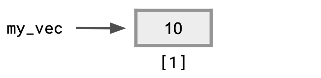
Suppose we have assigned a value of 10 to an object my_vec.
my_vec <- 10Then a is a vector containing one element, whose value is 10.
my_vec## [1] 10The [1] 10 appearing as the output states exactly that.
Visually, this looks like:
The way we access an element of a vector is to state the position of the element in the sequence comprising the vector inside square brackets and attach it after the name of the vector.
So, let us see what my_vec[1] returns.
The expression means to refer to the first element of my_vec, which we know to be 10.
my_vec[1]## [1] 10Wait a second, it still says [1] 10!
Because a vector is the most primitive information structure that R uses, there is no smaller structure.
This means that you can apply [1] as many times you want to a.
my_vec[1][1]## [1] 10
my_vec[1][1][1]## [1] 10
my_vec[1][1][1][1]## [1] 10
my_vec[1][1][1][1][1]## [1] 10Since the number inside the brackets specifies a position, you can try a number other than 1.
It is only that in the case of a, positions other than 1 do not exist.
my_vec[2]## [1] NA
my_vec[0]## numeric(0)What are these?
NA is short-hard for “not available” and means that there is no such thing.
numeric(0) means that it is a vector with no elements.
Once you get to length 0, [1] becomes NA but [0] produces numeric(0).
numeric(N) with N produces a sequence having length N where each element is 0.
Here is an example which creates a vector of five 0s.
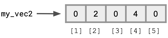
my_vec2 <- numeric(5)We can examine its contents and even change the values.
Below we change the values of my_vec2 at positions 2 and 4 to 2 and 4, respectively.
my_vec2[2] <- 2
my_vec2[4] <- 4
my_vec2
## [1] 0 2 0 4 0Here is a visualization of the situation.
Let’s play with these vectors a bit more.
In addition to specify a single position, you can give a range of positions, “from here to there”.
The syntax for a range specification is FROM:TO where FROM is the starting position and TO is the ending position.
The code below changes the values for the 5 positions of series_n and then provides examples of some range indexing.
my_vec2[1] <- 1
my_vec2[3] <- 3
my_vec2[5] <- 5
my_vec2[1:5]
## [1] 1 2 3 4 5
my_vec2[2:4]## [1] 2 3 4
my_vec2[2:2]## [1] 2If the END value is smaller than the START value, the elements appear in the reverse order.
my_vec2[4:1]## [1] 4 3 2 1You can use the negative sign in the range and position specification.
The - sign means “all positions other than”.
If the negative sign appears with the FROM or the TO index, then the other index must have the negative sign.
In the case of the negative ranging, the order between FROM and TO does not matter.
my_vec2## [1] 1 2 3 4 5
my_vec2[-3]## [1] 1 2 4 5
my_vec2[-2:-4]## [1] 1 5
my_vec2[-4:-2]## [1] 1 5
1.4.2 The combine function
We can create sequences with element specification.
The creation of this uses the function c, which means to “combine”.
The syntax is quite simple.
Within the parentheses following the initial c, state the elements of the series with a comma in between.
c(6, 2, 3)## [1] 6 2 3
c("data", "science", "rocks", "my", "socks")## [1] "data" "science" "rocks" "my" "socks"
c(3.0, 4.0, 2.0, 2.2, -4.5, -25.7)## [1] 3.0 4.0 2.0 2.2 -4.5 -25.7Using the c construction, you can obtain a subseries of a mother sequence with specific positions.
my_vec2[c(1,3,4)]## [1] 1 3 4
my_vec2[c(4,4,3,3,5,3,5,3)]## [1] 4 4 3 3 5 3 5 3R retrieves the elements individually, and whether the numbers repeat or whether the numbers are in order do not matter.
1.4.3 Element-wise operations
Let us look at the combine function more closely. We can define two sequences having the same lengths using the combine function.
A very common and useful set of operations when working with vectors are known as element-wise operations, which work on each element of a vector. Here is an example with element-wise addition.
a + 1/2## [1] 2.5 3.5 4.5 5.5 1.5 6.5To explain what happened, here is a visualization.
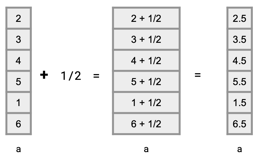
We can also apply element-wise subtraction, multiplication, division, and remainder.
a - 7## [1] -5 -4 -3 -2 -6 -1
a * 3## [1] 6 9 12 15 3 18
b / 2## [1] 4.5 4.0 3.5 0.5 1.0 0.5
b %% 3## [1] 0 2 1 1 2 1These element-wise operations can be applied to two sequences that have the same length.
a + b## [1] 11 11 11 6 3 7
a - b## [1] -7 -5 -3 4 -1 5
a * b## [1] 18 24 28 5 2 6
a / b## [1] 0.2222222 0.3750000 0.5714286 5.0000000 0.5000000 6.0000000
a %% b## [1] 2 3 4 0 1 0You can access some properties of the vector.
length, max, and min provide the length of a vector, the maximum among the elements in a vector, and the minimum among the elements in it, respectively.
length(a)## [1] 6
max(a)## [1] 6
min(a)## [1] 1In the case of numbers, the summation of all elements is possible.
sum(a)## [1] 21Another important feature of the function c is you can connect two vectors with c.
Here we recall the vectors a and b from earlier and then present the difference between the component-wise addition a + b and the sequence connection c(a, b).
c(a, b)## [1] 2 3 4 5 1 6 9 8 7 1 2 1Since a single value is a vector, connecting a vector with a conspicuously single value are actually vector concatenation.
c(a, 10)## [1] 2 3 4 5 1 6 10
c(78, a)## [1] 78 2 3 4 5 1 6You can connect more than two elements.
c(79, a, 17)## [1] 79 2 3 4 5 1 6 171.4.4 Booleans and element-wise operations
Not only can we apply mathematical operations but also we can apply comparisons.
a > b## [1] FALSE FALSE FALSE TRUE FALSE TRUE
a >= 3## [1] FALSE TRUE TRUE TRUE FALSE TRUEOnce you have a sequence of boolean whose length is equal to the vector at hand, you can use that boolean sequence (or vector) to select elements to generate subvectors.
a[a > b]## [1] 5 6
a[a >= 3]## [1] 3 4 5 6We can also use element-wise comparisons to count the number of occurrences of a certain element in a vector. For instance, consider this vector of greetings.
greetings <- c("hello", "goodbye", "hello", "hello", "goodbye")We can count the number of hello’s that occur as follows.
greetings == "hello"## [1] TRUE FALSE TRUE TRUE FALSE
sum(greetings == "hello")## [1] 31.4.5 Functions on numeric vectors
R provides programmers with convenient and powerful functions for creating and manipulating vectors.
The mean of a collection of numbers is its average value: the sum divided by the length.
Each of the examples below performs a computation on the vector called temps.
## [1] 6
sum(temps)## [1] 468
mean(temps)## [1] 78The diff function computes the difference between each adjacent pair of elements in an array.
The first element of the diff is the second element minus the first.
diff(temps)## [1] 0.0 -21.0 23.5 -24.5 5.5Following are some more commonly used functions that work over vectors. Learning this vocabulary is an important part of learning R, so refer to this list often as you work through examples and problems.
Please note: you do NOT need to memorize these!
Each of these functions takes some vector x as an argument and returns a single value.
| Function | Description |
|---|---|
sum(x) |
Add elements together |
prod(x) |
Multiply elements together |
all(x) |
Test whether all elements are true values |
any(x) |
Test whether any elements are true values |
sum(x != 0) |
Number of non-zero elements |
Each of these functions takes some vector x as an argument and returns a vector of values.
| Function | Description |
|---|---|
diff(x) |
Difference between adjacent elements |
round(x) |
Round each number to nearest integer |
cumprod(x) |
For each element, multiply all elements so far (cumulative product) |
cumsum(x) |
For each element, add all elements so far (cumulative sum) |
exp(x) |
Computes the exponential function |
log(x) |
Computes the natural logarithm of each element |
sqrt(x) |
Computes the square root of each element |
sort(x) |
Sort the elements |
Working with character vectors
The stringr package from the tidyverse provides us a collection of useful functions for working with character vectors. Here, we show some examples. We will study these in greater detail in a following section.
The name letters is a part of stringr and is a character vector containing the letters of the English alphabet.
letters## [1] "a" "b" "c" "d" "e" "f" "g" "h" "i" "j" "k" "l" "m" "n" "o" "p" "q" "r" "s"
## [20] "t" "u" "v" "w" "x" "y" "z"We saw in a previous section that the function str_c concatenates strings together. It can also be used element-wise to append some string to each element of a character vector.
str_c(letters, "end")## [1] "aend" "bend" "cend" "dend" "eend" "fend" "gend" "hend" "iend" "jend"
## [11] "kend" "lend" "mend" "nend" "oend" "pend" "qend" "rend" "send" "tend"
## [21] "uend" "vend" "wend" "xend" "yend" "zend"As we will see, all stringr functions can be used element-wise.
When the collapse argument is set, str_c combines output into a single string. By setting it to the empty string (""), the letters vector can be collapsed into one continuous string.
alphabet_string <-str_c(letters, collapse = "")
alphabet_string
## [1] "abcdefghijklmnopqrstuvwxyz"The str_length function inquires the length of a string.
str_length(alphabet_string)## [1] 26That’s the number of characters in the English alphabet!
When used element-wise, the function outputs the length of each string in a vector.
str_length(letters)## [1] 1 1 1 1 1 1 1 1 1 1 1 1 1 1 1 1 1 1 1 1 1 1 1 1 1 1A similar function, str_count, counts the occurrence of some pattern. We can confirm that only one “b” exists in the English alphabet.
str_count(letters, "b")## [1] 0 1 0 0 0 0 0 0 0 0 0 0 0 0 0 0 0 0 0 0 0 0 0 0 0 0We could replace the lowercase “b” with its uppercase counterpart. We first generate a Boolean vector that selects elements from letters that are equal to “b” and then provide the replacement with an assignment.
letters[letters == "b"] <- str_to_upper("b")
letters
## [1] "a" "B" "c" "d" "e" "f" "g" "h" "i" "j" "k" "l" "m" "n" "o" "p" "q" "r" "s"
## [20] "t" "u" "v" "w" "x" "y" "z"Alternatively, the stringr function str_replace_all can be used to provide one or more replacements.
str_replace_all(alphabet_string, c("b" = "B", "c" = "C"))## [1] "aBCdefghijklmnopqrstuvwxyz"The stringr function str_split divides a string into multiple segments. For example, it can split the alphabet string into two parts at the letter “g”.
str_split(alphabet_string, "g")## [[1]]
## [1] "abcdef" "hijklmnopqrstuvwxyz"The output returned is in the form of a list, which we haven’t seen before! We will cover lists in the next section.
A full cheat sheet of stringr functions can be found here, but listed below are some of the commonly used ones. The list includes several functions that we have not gone over yet.
Following are functions that take a character vector x as an argument and return a vector.
| Function | Description |
|---|---|
str_to_lower(x) |
Lowercase each element |
str_to_upper(x) |
Uppercase each element |
str_trim(x) |
Remove spaces at the beginning and/or end of each element |
The following function takes a character vector x with additional arguments, but also returns a vector.
| Function | Description |
|---|---|
str_sub(x, start, end) |
Extracts a substring from x given by start position and end position |
str_detect(x, "[:alpha:]") |
Whether each element is only letters (no numbers or symbols) |
str_detect(x, "[:digit:]") |
Whether each element is only numeric (no letters) |
The following functions take both a character vector x and a pattern string to search for.
Pattern strings can be more general like "[:alpha:]" or "[:digit:]" from the above list (these are also called regular expressions or RegEx for short, which we won’t cover in detail :-).
Each of these functions returns a vector.
| Function | Description |
|---|---|
str_count(x, pattern) |
Count the number of times a pattern appears among the elements of an array |
str_which(x, pattern) |
The indexes of vector x where the pattern is found |
str_replace_all(x, pattern) |
Replace all matched patterns in each string |
str_detect(x, ^pattern) |
Whether each element starts with the pattern |
The following function also takes a vector x of strings and a pattern string.
However, unlike the above table, this function returns a list.
| Function | Description |
|---|---|
str_locate_all(x, pattern) |
The positions within each element that a pattern is found |
str_split(x, pattern) |
Split each string into a varying number of pieces |
The following function is a helpful diagnostic tool to view matched patterns.
| Function | Description |
|---|---|
str_view(x, pattern) |
Visualizes all pattern matches in vector x
|
1.5 Lists
Like vectors, lists also group values together. However, unlike vectors, lists can hold values that are of different types. For instance:
mixed <- list("apple", 1.5, 2L, TRUE)
mixed
## [[1]]
## [1] "apple"
##
## [[2]]
## [1] 1.5
##
## [[3]]
## [1] 2
##
## [[4]]
## [1] TRUEIt can be helpful to examine the structure inside the list.
We use str for this.
str(mixed)## List of 4
## $ : chr "apple"
## $ : num 1.5
## $ : int 2
## $ : logi TRUELists hold just about anything; they can even contain vectors…
## List of 3
##  $ : chr [1:3] "asparagus" "arrowroot" "tomato"
##  $ : chr [1:2] "mango" "kumquat"
##  $ : num 3.14
…or more lists!
## List of 3
##  $ :List of 2
##   ..$ : num 1
##   ..$ : num 1
##  $ :List of 3
##   ..$ : num 2
##   ..$ : num 2
##   ..$ : num 2
##  $ : chr "hello world"
1.5.1 Working with lists
Let’s examine the mixed2 list more closely.
mixed2## [[1]]
## [1] "asparagus" "arrowroot" "tomato"
##
## [[2]]
## [1] "mango" "kumquat"
##
## [[3]]
## [1] 3.14159[ extracts a sub-list.
The result is always a list.
str(mixed2[2])## List of 1
## $ : chr [1:2] "mango" "kumquat"We can also subset a list the same way we do with vectors. Remember that the result is still a list.
str(mixed2[1:2])## List of 2
## $ : chr [1:3] "asparagus" "arrowroot" "tomato"
## $ : chr [1:2] "mango" "kumquat"If we wish to extract the vector inside mixed2[2], we must use [[.
This extracts a single component from a list.
We can use it to retrieve, for example, the vector of fruits:
mixed2[[2]]## [1] "mango" "kumquat"What if we only wanted the mango?
mixed2[[2]][1]## [1] "mango"Yum!
1.5.2 Visualizing lists
The difference between [ and [[ is important, but too easy to confuse.
The following visual will clarify the point.
Suppose that we have the following list a.
Then we can imagine operations on a as the following:
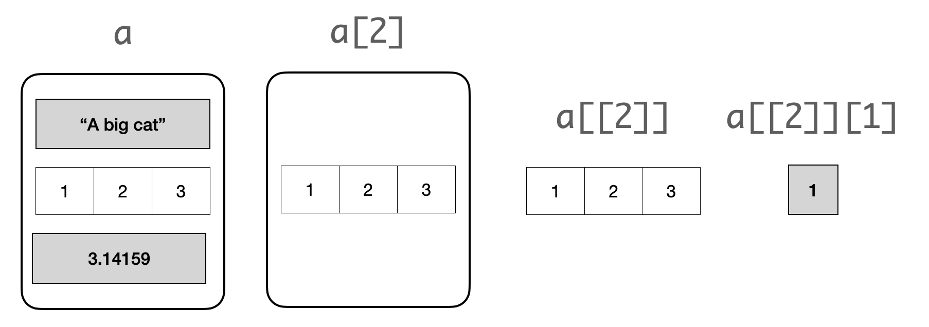
-
ais a list -
a[2]is also a list, this time containing a single element -
a[[2]]is the second component of the list, a vector -
a[[2]][1]is the first element of that vector
Groovy! The “pepper shaker photos” in R for Data Science provides another nice visualization of the different ways we can extract pieces from a list.
1.6 stringr Operations
As we mentioned earlier, tidyverse is a collection of packages.
One of the packages tidyverse contains is stringr, which offers a variety of methods for manipulating strings.
Just as a single number can be seen as a vector containing one number, a single string can be viewed as a vector containing one string.
So, applying a function to a string is the same as applying a function to a string vector.
Depending on what we are interested in doing, we can classify the functions in stringr into the following categories:
- Detect Matches: finding and locating matches of a pattern in each string in a string vector
- Subset Strings: Extracting subtrings and subvectors from a string vector matching a pattern
- Manage Lengths: Inquiring about the lengths and padding/trimming the strings
- Mutate Strings: Mutating the strings appearing in a string vector
- Join and Split: Changing the structure of a vector
- Order Strings: Sorting
Be sure to bookmark the stringr cheatsheet.
1.6.2 Regular expressions
The pattern matching functions of stringr accept regular expressions.
A regular expression is a string that specifies a collection of strings in a possibly compact manner.
Here are some examples of regular expressions and how one of the stringr functions str_detect uses it find patterns in string vector c("May 17, 2019", "Certified mail", "FL 33333", "Oppa Locka", "to Mr. Haan", "arrived").
The function str_detect receives two arguments.
The first is a string (or a string vector) and the second is the pattern.
The function returns for each element in the vector, whether the pattern appears.
Let us first define a string vector with the six elements.
s <- c("May 17, 2019", "Certified mail", "FL 33333",
       "Oppa Locka", "to Mr. Haan", "arrived")
s
## [1] "May 17, 2019" "Certified mail" "FL 33333" "Oppa Locka"
## [5] "to Mr. Haan" "arrived"Now you see a bracket with a number other than 1.
The [5] states that “to Mr. Haan” is the fifth element of the vector.
The pattern strings appearing in the following have the following meaning
| pattern | meaning |
|---|---|
"a" |
any appearance of “a” |
"a[iy]" |
any “a” then one of “i” or “y” |
"a$" |
“a” at the end of string |
"^a" |
“a” at the start of string |
"^a.*d$" |
“a” at the start, any string, and then a “d” at the end |
"ppa" |
“ppa” |
"3{4}" |
“3” repeated four times in sequence |
"[aeiou].[aeiou]" |
one from “aeiou”, some character, and one from “aeiou” |
s## [1] "May 17, 2019" "Certified mail" "FL 33333" "Oppa Locka"
## [5] "to Mr. Haan" "arrived"
str_detect(s, "a")## [1] TRUE TRUE FALSE TRUE TRUE TRUE
str_detect(s, "a[iy]")## [1] TRUE TRUE FALSE FALSE FALSE FALSE
str_detect(s, "a$")## [1] FALSE FALSE FALSE TRUE FALSE FALSE
str_detect(s, "^a")## [1] FALSE FALSE FALSE FALSE FALSE TRUE
str_detect(s, "^a.*d$")## [1] FALSE FALSE FALSE FALSE FALSE TRUE
str_detect(s, "ppa")## [1] FALSE FALSE FALSE TRUE FALSE FALSE
str_detect(s, "3{4}")## [1] FALSE FALSE TRUE FALSE FALSE FALSE
str_detect(s, "[aeiou].[aeiou]")## [1] FALSE TRUE FALSE FALSE FALSE TRUESo, the syntax is:
- use the square brackets to specify a list of characters
- use the curly brackets to specify the number of repetitions
- use the period to specify any character
- use the caret
"\^"and the dollar sign to specify the start and the end of string, respectively - use
\*to specify any number of repetitions, including 0 repetitions.
A useful diagnostic tool to visualize matches against a pattern is the function str_view, which highlights any matches hit by the regular expression. For instance:
str_view(s, "[aeiou].[aeiou]", html = TRUE)In the square brackets you can specify a range using a dash and the caret to mean “not”. By putting a pair of numbers inside a pair of curly brackets, you can specify a permissible range of the number of repetitions.
The patterns below mean the following:
| pattern | meaning |
|---|---|
"[a-z]" |
“a” through “z” at least one |
"[A-Z]{2,5}" |
“A” through “Z” between 2 and 5 times |
"[^a-zA-Z]" |
a non-alphabet |
"[0-9]" |
a numeral |
s## [1] "May 17, 2019" "Certified mail" "FL 33333" "Oppa Locka"
## [5] "to Mr. Haan" "arrived"
str_detect(s, "[a-z]")## [1] TRUE TRUE FALSE TRUE TRUE TRUE
str_detect(s, "[A-Z]{2,5}")## [1] FALSE FALSE TRUE FALSE FALSE FALSE
str_detect(s, "[^a-zA-Z]")## [1] TRUE TRUE TRUE TRUE TRUE FALSE
str_detect(s, "[0-9]")## [1] TRUE FALSE TRUE FALSE FALSE FALSE1.6.3 Detect matches
There are functions in this category.
-
str_detect(STRING, PATTERN): As we have seen previously, the function returns a vector of boolean representing whether the elements ofSTRINGmatchingPATTERN. -
str_which(STRING, PATTERN): The function works likestr_detectbut instead of boolean vector, returns the indexes at which the pattern appears; in other words, at which indexes, the value ofstr_detect(STRING, PATTERN)is true. -
str_count(STRING, PATTERN): The function returns for each element ofSTRING, at how many different positions the pattern aligns. -
str_locate(STRING, PATTERN): The function finds for each element ofSTRING, the first (or the closest to the start of string) match of the pattern and provides the start and end character positions of the first match as a pair of integers (that is, a length-2 vector of integers). If there are no matches for an element ofSTRING, the function returns a pair ofNA.
Let us recall s.
s## [1] "May 17, 2019" "Certified mail" "FL 33333" "Oppa Locka"
## [5] "to Mr. Haan" "arrived"Here is the result of finding “[0-9]” in the strings.
str_which(s, "[0-9]")## [1] 1 3Here is finding one of “aeiou” and any alphabet and counting the occurrences.
Note that in “to Mr. Haan” there are two places that match the pattern "[aeiou][A-Za-z]", that is “aa” and “an”.
The pattern counting goes by repeating the action of finding the first match and then asserting the characters leading to the end of the match unusable for finding matches.
With the feature, after finding the first, “aa”, the prefix “to Mr. Haa” is no longer available, and so “an” does not qualify as a match.
str_count(s, "[aeiou][A-Za-z]")## [1] 1 4 0 1 1 3So, if we find three numerals in sequence with no gap, the elements 1 and 3 have exactly one match each, though there are multiple possibilities for aligning the pattern.
str_count(s, "[0-9]{3}")## [1] 1 0 1 0 0 01.6.4 Subset strings
Here are the functions in this category.
-
str_sub(STRING, START, END): Creates a new vector consisting of the substrings of the elements ofSTRINGwithSTARTandENDas the staring and ending positions, respectively. -
str_subset(STRING, pattern): Creates a new vector keeping only those elements insmatching the pattern. -
str_extract(STRING, pattern): The same asstr_subsetconcerning what to find, but the function returns a table not a one-dimensional vector. See the examples below to examine the differences amongstr_subset,str_extract, andstr_match.
str_sub(s, 4, 7)## [1] " 17," "tifi" "3333" "a Lo" "Mr. " "ived"
str_subset(s, "[a-zA-Z][^a-zA-Z]+[a-zA-Z]")## [1] "Certified mail" "Oppa Locka" "to Mr. Haan"
str_extract(s, "[a-zA-Z][^a-zA-Z]+[a-zA-Z]")## [1] NA "d m" NA "a L" "o M" NA
str_match(s, "[a-zA-Z][^a-zA-Z]+[a-zA-Z]")## [,1]
## [1,] NA
## [2,] "d m"
## [3,] NA
## [4,] "a L"
## [5,] "o M"
## [6,] NABoth str_extract and str_match have their version for “apply to all matches”, like str_locate_all. Their names are str_extract_all and str_match_all.
1.6.5 Manage lengths
The following functions belong to this category.
-
str_length(STRING): Returns the length of each element. -
str_pad(STRING, WIDTH, side=OPTION, pad=X):Appends the stringXto both or either side of each element ofSTRINGas many times as necessary so as to inflate the length of element to at leastWIDTH. TheOPTIONis one of"left","right", and"both"to indicate where the padding should occur. They respectively represent “the left side only”, “the right side only”, and “both sides so as to center the original”. If the original has length greater than or equal toWIDTHno padding occurs. In the case of “both”, if the number of necessary padding is an odd number to make the length equal toWIDTH, the right side receives one more than the left side. The padding stringXmust be a single character. You may omit the specification partpad=inpad=X. -
str_trunc(STRING, WIDTH, side=OPTION, ellipsis=E): This is in some sense at the opposite ofstr_pad. The function shrinks each string to lengthWIDTHwith the single-character stringEfor replacement. Theside=specification states where the replacement occurs and should be one of"left","right", and"center". You may omit theellipsis=prefix. -
str_trim(STRING, side=OPTION): Trims the white space at the end. The option value is one of"left","right", and"both", which correspond to “the left side only”, “the right side only”, and “both sides”.
str_length(s)## [1] 12 14 8 10 11 7
str_pad(s, 11, side="both", pad=".")## [1] "May 17, 2019" "Certified mail" ".FL 33333.." "Oppa Locka."
## [5] "to Mr. Haan" "..arrived.."
str_pad(s, 10, side="left", ".")## [1] "May 17, 2019" "Certified mail" "..FL 33333" "Oppa Locka"
## [5] "to Mr. Haan" "...arrived"
str_trunc(s, 3, side="right", ellipsis="_")## [1] "Ma_" "Ce_" "FL_" "Op_" "to_" "ar_"
str_trunc(s, 5, side="center", "#")## [1] "Ma#19" "Ce#il" "FL#33" "Op#ka" "to#an" "ar#ed"
str_trim(" abc ", side="right")## [1] " abc"
str_trim(" abc ", side="both")## [1] "abc"1.6.6 Mutate strings
The first three functions execute substitutions to parts of each string.
-
str_sub() <- VALUE: Here thestr_sub()part follows the syntax of the method we earlier discussed - the substrings with specific range of indexes inside strings. After this action, each substring will becomeVALUE.s <- c("5/17/2019", "Certified mail", "FL 33333", "Oppa Locka", "to Mr. Haan", "arrived")Since the
str_sub() <- VALUEmodifies the original, let us copystoscopyand then execute the action on the copy, not the original. In that manner, we can preserve the original. Note the use of 0 and 0 in the second instance, the position range of 0 through 0 corresponds to the part before the start of the string.scopy <- s str_sub(scopy, 1, 3) <- "I am " scopy## [1] "I am 7/2019" "I am tified mail" "I am 33333" "I am a Locka" ## [5] "I am Mr. Haan" "I am ived"scopy <- s str_sub(scopy, 0, 0) <- "I am " scopy## [1] "I am 5/17/2019" "I am Certified mail" "I am FL 33333" ## [4] "I am Oppa Locka" "I am to Mr. Haan" "I am arrived"s## [1] "5/17/2019" "Certified mail" "FL 33333" "Oppa Locka" ## [5] "to Mr. Haan" "arrived" str_replace(STRING, PATTERN, REPLACEMENT): Replaces the first occurrence ofPATTERNwithREPLACEMENT.-
str_replace_all(STRING, PATTERN, REPLACEMENT): Replaces all occurrences ofPATTERNwithREPLACEMENT. Likestr_locate_allthe function finds a set of non-overlapping occurrences and then replaces all the occurrences it has identified.Both functions return the vector resulting from their action. The original remains intact.
t <- s
str_replace(t, "a", "oo")
## [1] "5/17/2019" "Certified mooil" "FL 33333" "Oppoo Locka" ## [5] "to Mr. Hooan" "oorrived"t <- s str_replace_all(s, "a", "oo")## [1] "5/17/2019" "Certified mooil" "FL 33333" "Oppoo Lockoo" ## [5] "to Mr. Hoooon" "oorrived"t <- s str_replace_all(s,"[0-9][0-9]", "##")## [1] "5/##/####" "Certified mail" "FL ####3" "Oppa Locka" ## [5] "to Mr. Haan" "arrived"
There are three more string mutation functions.
str_to_lower(STRING): This converts each uppercase letter to its corresponding lowercase letter.str_to_upper(STRING): This converts each lowercase letter to its corresponding uppercase letter.-
str_to_title(STRING): This converts each string to a title-like format.Each of the three methods returns a new vector.
t <- s
str_to_lower(s)
## [1] "5/17/2019" "certified mail" "fl 33333" "oppa locka" ## [5] "to mr. haan" "arrived"t <- s str_to_upper(s)## [1] "5/17/2019" "CERTIFIED MAIL" "FL 33333" "OPPA LOCKA" ## [5] "TO MR. HAAN" "ARRIVED"t <- s str_to_title(s)## [1] "5/17/2019" "Certified Mail" "Fl 33333" "Oppa Locka" ## [5] "To Mr. Haan" "Arrived"
1.6.7 Join and split
We only show two functions in this category.
-
str_dup(STRING, TIMES): Create from a vectorSTRING, a new vector where each element appears consecutively, without a gap,TIMEStimes. -
str_c(STRING): Collapse the elements column-wise into a single dimensional vector. -
str_c(STRING, collapse=X): Concatenate the elements column-wise withXin between and then concatenate the elements row-wise withXin between, thereby generating a single-element vector.
Below are examples.
t <- s
str_dup(t, 3)
## [1] "5/17/20195/17/20195/17/2019"
## [2] "Certified mailCertified mailCertified mail"
## [3] "FL 33333FL 33333FL 33333"
## [4] "Oppa LockaOppa LockaOppa Locka"
## [5] "to Mr. Haanto Mr. Haanto Mr. Haan"
## [6] "arrivedarrivedarrived"
str_c(t)## [1] "5/17/2019" "Certified mail" "FL 33333" "Oppa Locka"
## [5] "to Mr. Haan" "arrived"
str_c(t, collapse=":")## [1] "5/17/2019:Certified mail:FL 33333:Oppa Locka:to Mr. Haan:arrived"1.6.8 Sorting
There are two functions.
-
str_sort(STRING,decreasing=X,na_last=Y,numeric=Z): Sorts the elements as the string. The arguments after the first one are optional.X,Y, andZare boolean. Withdecreasing=TRUEthe ordering is reverse. Thena_last=FALSE, allNAmove to the start. Withnumeric=TRUE, the function treats numerical sequences as numbers; otherwise, it treats them as character sequences. -
str_order(...): The same arguments asstr_sort, but instead of actually sorting, returns the sequence of indexes such that ordering the elements according to the index list produces the same result asstr_sort.
## [1] "5/17/2019"      "arrived"        "Certified mail" "FL 33333"
## [5] "Oppa Locka" "to Mr. Haan"## [1] "to Mr. Haan" "Oppa Locka" "FL 33333" "Certified mail"
## [5] "arrived" "5/17/2019"## [1] 5 4 3 2 6 1
1.6.9 An example: stringr and lists
We end this section with an educational example of when you might need to work with the stringr package.
Recall that str_locate_all is a method for working with strings; it returns the positions within each element that a pattern string is found as a list.
Let’s try to use what we know to extract common bird names.
birds <- c("Black-crowned Night-Heron-Nycticorax",
           "Little-egret-Egretta garzetta")
The common names are Black-crowned Night-Heron and Little-egret.
We can extract this by looking for the last occurrence of the dash (-).
Here they are:
str_view(birds, "-", html=TRUE)The str_locate_all function can tell us the starting and ending positions of all occurrences of the dash.
dash_positions <- str_locate_all(birds, "-")
dash_positions
## [[1]]
##      start end
## [1,]     6   6
## [2,]    20  20
## [3,]    26  26
##
## [[2]]
## start end
## [1,] 7 7
## [2,] 13 13As expected, we have a list.
Let’s first examine the results for the Night Heron, which are stored at index 1 of this list.
We now know that to pluck out these results we must use [[.
dash_positions[[1]]## start end
## [1,] 6 6
## [2,] 20 20
## [3,] 26 26Congrats – we’re out of the list! What we have now is three vectors sandwiched together into one, one for each occurrence of the dash. We are only interested in the last one.
tail is a handy function for extracting the last value of a vector.
tail(dash_positions[[1]], n=1) # why n = 1? why not 2?## start end
## [3,] 26 26Technically, we only care about the ending position of the dash (at index 2) but either value will do.
last_dash <- tail(dash_positions[[1]], n=1)[1]
last_dash
## [1] 26We’re almost done: we now know that the common name occurs between positions 1 and 25 (why not 26?). We can use str_sub to extract the substring.
str_sub(birds[1], end = last_dash - 1)## [1] "Black-crowned Night-Heron"Here is everything together:
dash_positions <- str_locate_all(birds, "-")
last_dash <- tail(dash_positions[[1]], n=1)[1]
str_sub(birds[1], end = last_dash - 1)
## [1] "Black-crowned Night-Heron"What would the answer be for extracting Little-egret? Try it out!
1.7 Exercises
Be sure to install and load the following packages into your R environment before beginning this exercise set.
Question 1. Let us explore the limit of the double data type. According to the textbook, the largest double value is greater than or equal to 1.79e+308. Can you find the largest digit \(d\) (d must be one of \(\{0..9\}\)) such that 1.79de+308 is not Inf? Let us do this with a simple trial. Type 1.79de+308 with the d substituted with the values \(0, 1, 2, 3, ...\) in this order, and stop when the value presented after pressing the return key becomes Inf.
After examining the values, store in a variable the_digit the value of d you have found.
Question 2. Let us learn how to convert data types. Recall as.character, as.double, and as.integer convert a given value to a string, a double, and an integer, respectively. We can also test to see if a value is a certain data type by replacing as with is. Recall also that to specify a string with its character sequence we can use either a matching pair of double quotation marks or a matching pair of single quotation marks sandwiching the sequence.
Following is a string called a_happy_string and a double named double_trouble:
a_happy_string <- "-4.5"
double_trouble <- 81.9
Here are some findings based on the above functions. Which of the following statements are TRUE?
as.double(a_happy_string) produces an error because we cannotcovert a string to a double.
2.
as.integer(a_happy_string) returns the value \(-4.5\).3.
as.character(double_trouble) returns the value \("81.9"\).4.
is.integer(1) returns TRUE.Question 3. Let us extract some information from strings. Following are three strings stored in three separate names.
str1 <- "State"
str2 <- "Department"
str3 <- "Office"
Do the following three tasks with these three strings:
- Inquire the length of each string, and store the three length values to
l1,l2, andl3, respectively. - Connect the three strings in the order of
str1,str2, andstr3usingstr_candstr_cwithsep = " ", and store the two results injoin1andjoin2. - Obtain the substrings of
join1between position pairs \((4,10)\), \((-7, -1)\), and \((8, 8)\). Store the substrings insub1,sub2, andsub3, respectively.
Question 4. Let us execute some operations to generate Boolean values. Use two variables val1 and val2 and assign them to the values 12.3 and 45.6, respectively. Then put the two values in the six comparisons “equals”, “not equals”, “greater than”, “greater than or equal to”, “less than”, and “less than or equal to”. Store the six results in the variables test1, test2, test3, test4, test5, and test6, respectively.
Question 5. Let us play with Boolean operations. Let str4 be a string variable. Assign the value of hammerhead to str4. Then create three Boolean variables check1, check2, and check3 and assign, to these variables, the results of testing if the length of str4 is equal to 10, if the length of str4 is less than 5, and if the substring of str4 from positions 10 to 10 is equal to "a". Print the three Boolean value, and then compute the “or” of the three values and the “and” of the three values, and store these results in the names the_OR and the_AND, respectively.
Question 6. Suppose we have three Boolean names tf1, tf2, and tf3. Suppose we assign the following eight value pairs to them.
-
FALSE,FALSE, andFALSE -
FALSE,FALSE, andTRUE -
FALSE,TRUE, andFALSE -
FALSE,TRUE, andTRUE -
TRUE,FALSE, andFALSE -
TRUE,FALSE, andTRUE -
TRUE,TRUE, andFALSE -
TRUE,TRUE, andTRUE
Answer the value of tf1 | !tf2 & tf3 in the four combinations, and store them in eight names bool1, bool2, …, bool8.
Question 7. Following are three Boolean expressions that evaluate to either TRUE or FALSE. Explain every step in the evaluation process before TRUE or FALSE is ultimately returned.
(2 - 1) == ((TRUE == TRUE) != FALSE)
(10 - (FALSE/2 + max(TRUE, FALSE))) >= (TRUE + 1)
(Inf > 5) == ((Inf > Inf) | (Inf >= Inf))
Question 8. A student is diligently studying Boolean data types and is stumped by the following:
I don’t understand why
"Zoo" > "Napping"isTRUEwhen “Napping” has more characters than “Zoo”. But when I do"ZZZ" > "ZZZping", it returnsFALSEwhich makes sense because “ZZZping” has more characters than “ZZZ”. So shouldn’t the first expression evaluate toFALSEas well for the same reason2 > 5isFALSE?
What would you tell this student? Should we file a bug report to the R maintainers?
Question 9. Suppose we have four names s1, s2, s3, and s4 that are defined as follows:
s1 <- "Fine"
s2 <- "Dine"
s3 <- "Sine"
s4 <- "Wine"
We then apply the following function and store the result in the name snew:
snew <- str_c(s1, s2, s3, s4, sep = " ")
snew
## [1] "Fine Dine Sine Wine"Question 9.1 What is the length of
snew? Do not compute this manually! Use an R function. Store your answer in the namesnewlen.Question 9.2 How many times does
"in"appear insnew? You may find this manually or by using an R function. Assign your answer to the nameintimes.Question 9.3 Recall
str_sub( snew, a, b)fromstringrproduces the substring ofsnewfrom positionato positionb. Answer the combination ofaandbthat produces"in"such thatais the largest. This is also sometimes called a “right find” because the search is done from the right rather than the left. Store the combination ofaandbyou found in the namesaandb.
Question 10: Vector manipulations. In this exercise we practice some basic construction and manipulation of vector data types.
Question 10.1. Form a vector that contains the numbers 3, \(\pi\), 4, 9, and \(e\) (Euler’s constant), in that order. Your solution should reference the constants \(\pi\) and \(e\) without having to define them explicitly. Assign it to the name
vec1.Question 10.2. Form a vector that contains the nine strings
"Dear","string",",","this","is","much","ado","about", and" ". Note that the last element is a string containing a single whitespace. Name thisvec2.Question 10.3. Form a vector that appends
vec2aftervec1. Call itvec3. What is the data type of this new vectorvec3? Use an R function to determine this and assign that answer to the namevec3_type. Then observe the difference in data types betweenvec1,vec2, andvec3.
Question 11: Sequences. This exercise explores the use of vectors to form various sequences using the seq() function. Each of these questions should require only one line of code to compute the answer.
Question 11.1 Form a vector that generates a sequence of numbers from 0 to 20 in steps of 2, e.g., 0, 2, 4, 6, 8, …, 20. Assign this vector to the name
steps2.Question 11.2 Form a vector that generates a sequence containing multiples of 11 from 0 up to and including 1221. Assign this vector to the name
mult11.Question 11.3 Form a vector that generates a sequence containing the first 20 powers of 4, e.g., \(4^0 = 1\), \(4^1 = 4\), \(4^2 = 16\), etc. Assign your answer to the name
powers4.
Question 12: Element-wise operations. A benefit of working with vectors is that we can use vectors to accomplish element-wise operations, that is, some operation that is applied to every element of a vector. What makes element-wise operations attractive to use is that they can be applied with a single line of code. This exercise explores some element-wise operations.
-
Question 12.1 Let us compute the interest on several loans at once.
Question 12.1.1 The vector
bank_loansfrom the packageedsdatacontains 100,000 different loans. Assuming an annual simple interest rate of 4%, compute the amount each borrower would owe after one year if no payments were made during that time toward the loan. That means we can multiply the loan amount by \(1.04\) to get the amount owed after one year. Compute the amount owed for each loan inbank_loansafter one year. Assign your answer to the nameamount_owed.Question 12.1.2 What is the total amount of interest collected by the bank from all these loans after one year? Assign your answer to
total_interest_amount.
-
Question 12.2 Suppose the population of Datatopia is growing steadily at 3% annually. On 1/1/2021, Datatopia had 1,821,411,277 people. Calculate the expected population of the country for the next 20 years.
Question 12.2.1 Compute the expected population for the next 20 years as a 20-element vector, and store it in
p. You can do this by first creating a sequence of 20 values1..20, powering 1.03 with the 20 values, and multiplying it by the initial population.Question 12.2.2 Set
pop_2025andpop_2040to the population estimates for 2025 and 2040, respectively. Then setpop_2025_to_2040to a vector containing the estimates from 2025 to 2040 (the years 2025 and 2040 are both inclusive).-
Question 12.2.3 What happens when you try to access the following element in the vector
pop_2025_to_2040?pop_2025_to_2040[17]Are you surprised by the result? Should you expect an error when trying this? Why or why not?
Question 12.2.4 Set
pop_2025_to_2040_reverseto a vector containing the populations inpop_2025_to_2040, but in reverse order. That is, starting first from 2040 and ending with 2025. To do this, use an index sequence.Question 12.2.5 Suppose that our population estimates for the years 2033 and 2034 are too unreliable to be useful and we would like to raise this error somehow. Flag this error in
pop_2025_to_2040by setting the appropriate indices inpop_2025_to_2040toNA.NAis a special name that stands for “not a number”.Question 12.2.6 The numbers in
pop_2025_to_2040are large, which can sometimes be hard to interpret. Report the figures as numbers in billions instead. Accomplish this work using element-wise operation using a single line of R code and assign your answer to the namepop_2025_to_2040_billions.Question 12.2.7 How many years had a population exceeding 3 billion? Use your vector
pop_2025_to_2040_billionsto answer this. You will need to use another element-wise operation. Assign the number to the namemore_than_3_bill. If your answer is coming out asNA, be sure to read the help and look at any arguments you can use.
Question 13: Exploring stringr. We have already learned how to do basic tasks with strings like inquiring about the number of characters in the string and finding substrings. But data science work often involves doing much more advanced tasks, e.g., splitting strings, replacing certain characters that match some pattern, etc. The stringr package from the tidyverse brings a suite of modern tools to use for working with strings in data science. Let’s explore some of them in this second part. Be sure to bookmark its cheatsheet for reference.
bands is a character vector in the package edsdata that contains some band names.
Question 13.1 Obtain two copies of
bands, one with every character in uppercase (e.g., LIKE THIS) and another with every character in lowercase (e.g., like this). Store the results inupperandlower, respectively. Use astringrfunction.-
Question 13.2 Here is another character vector,
bird_in_a_hand, that looks a bit different frombands. Even though both are seen as character vectors in R, what is the difference betweenbird_in_a_handandbands?bird_in_a_hand <- c("b","i","r","d", "","i","n","","a","", "h","a","n","d") bird_in_a_hand## [1] "b" "i" "r" "d" "" "i" "n" "" "a" "" "h" "a" "n" "d" Question 13.3 Repeat Question 13.1, but for
bird_in_a_hand. Assign your answers to the namesupper_birdandlower_bird, respectively.-
Question 13.4 The
stringrfunctionstr_remove_all()can be used to remove matched patterns in a string. For instance, we could remove all lowercase a’s and b’s from the character vectorbird_in_a_handas follows:str_remove_all(bird_in_a_hand, "[ab]")Now take
bandsand modify it by removing each occurrence of a vowel in lowercase ('a', 'e', 'i', 'o', 'u'). Store the result indevoweled.
Question 14: Lists. This exercise gives practice with the list data type.
-
Question 14.1 Using the function
listcreate a listcourseswhose elements are"MTH118","GEG2490","CSC160","CSC353","ACC419","PSC356", and"BIL155". Then:- Sort the list using the function
str_sort()and store the result incourses_sorted. - Apply
str_subfrom position 4 to position 6 to the elements ofcoursesand applystr_sortto the result. Store it innumbers_sorted.
- Sort the list using the function
-
Question 14.2 The name
fruitsis a character vector with some fruits.fruits <- c( "apples and oranges and pears and bananas", "pineapples and mangos and guavas" )-
Question 14.2.1 Accomplish the following tasks:
Create a list
fruits_listfromfruitsusing thelistfunction.Create a vector
fruits_unlistedby applyingunlisttofruits_list.-
Try executing:
The middle one presents a warning message. Store the last result in
split_fruits. Print
split_fruits.
-
Question 14.2.2 Let’s recap what just happened:
- What is the difference between
fruits,fruits_list,fruits_unlisted, andsplit_fruits? Note the data type stored in each of these names (e.g., list, character vector, integer, etc.). - Why did you get a warning when trying
str_split(fruits_list, "[and]")? Read the help forstr_splitto help you answer this. - Why does the word “and” no longer appear in the elements inside
split_fruits?
- What is the difference between
-
Question 15: More stringr. Let’s return to stringr again, this time looking at a few more functions that work with regular expressions. We actually saw one already when we worked on “devoweling” band names. Be sure you have read the textbook section on stringr before continuing with this part.
As a real-world example, the name band_of_the_hour is a string about the “Band of the Hour” at the University of Miami. The string is available in the edsdata package.
-
Question 15.1 The function
str_match( s, p )finds the first occurrence of the patternpin the strings. Find the following patterns inband_of_the_hourusingstr_matchand store the results in variablesm1, …,m3:
"[A-Z]",2. any series of lowercase alphabetical characters
"[a-z]+",3. any numeral
"[0-9]".Question 15.2 Now use
str_match_all()to find the occurrences of the following two patterns and store them inma1andma2: (a) any series of numerals and (b) any word that begins with an uppercase letter (e.g., “Fiesta”, “Band”, “University”, etc.). Verify your answer by examining the contents ofma1andma2.Question 15.3 Now use
str_count()to count the occurrences of"Arrow"and store inarrow_countand then usestr_split()to splitband_of_the_hourat each white space and store it inband_of_the_hour_split.-
Question 15.4 The
stringrfunctionstr_subset()keeps strings that match a pattern. For example:str_subset(c("x", "y", "xx", "yy"), "x")Now answer how you might obtain the elements in the list
band_of_the_hour_splitthat have a"0"in it. Store the result inzero_elements.
Question 16. Suppose we have a vector of course IDs:
badly_formed_ids <- c("CSC_100", "BIO 111", "MTH161H",
                      "ECO--220", "MUS..160A")
badly_formed_ids
The school codes their IDs as follows:
- An ID starts with three uppercase letters.
- An ID has three numerals after the uppercase letters.
- Between the letters and the numerals, an ID may contain symbols that are neither letters nor numerals.
- An ID may have an additional alphabet character at the end.
Unfortunately, this format is not very good for data science. While it allows for a wide range of possible IDs, the flexibility is an obstacle to any analysis using R, e.g., how to tell which courses are offered through Computer Science (CSC)? How to find how many 200-level courses the school offers?
Let us “standardize” these course IDs into a uniform format consisting solely of the initial three letters followed by three numerals. After application of the function, the above IDs should look like:
c("CSC100", "BIO111", "MTH161", "ECO220", "MUS160")Answer how you might obtain this with a single line of R code using a single stringr function.