2 Data Transformation
The work of data science begins with a dataset. These datasets can be so large that any manual inspection or review of them, say using editing software like TextEdit or Notepad++, becomes totally infeasible. To overcome this, data scientists rely on computational tools like R for working with datasets. Learning how to use these tools well lies at the heart of data science and what data scientists do daily at their desks.
A part of what makes these tools so powerful is that we often need to apply a series of actions to a dataset. Data scientists talk a lot about the importance of data cleaning, stating that without data cleaning no data analysis results are meaningful. Some go further to say that the most important step in the data science life cycle is data cleaning because, from their point of view, the analysis process following data cleaning is a routine to a great degree. As such, another important aspect of working with datasets is transforming data, i.e., rendering data suitable for analysis. When data is made into an analysis-ready form, we call such data tidy data. Transforming data to become tidy data is the focus of this chapter.
The tools we will cover in this chapter to accomplish this goal are also key members of the tidyverse. One is called tibble, which is a data structure for managing datasets, and another is called dplyr, which provides a grammar of data manipulation for acting upon datasets stored as tibbles. We will also learn about a third called purrr to help with the data manipulations, e.g., say when a column of data is in the wrong units.
2.1 Datasets and Tidy Data
Data scientists prefer working with data that is tidy because it facilitates data analysis. In this section we will introduce a vocabulary for working with datasets and describe what tidy data looks like.
2.1.1 Prerequisites
As before, let us load tidyverse.
The tidyverse package comes with scores of datasets. By typing data() you can see a list of data sets available in the RStudio environment you are in. Quite a few data come with tidyverse. If your session has not yet loaded tidyverse, the list can be short.
2.1.2 A “hello world!” dataset
A dataset is a collection of values, which can be either a number or string. Let us begin by looking at our first dataset. We will examine the Motor Trend Car Road Test dataset which is made available through tidyverse. It was extracted from the 1974 Motor Trend US magazine, and contains data about fuel consumption and aspects of automobile design for 32 car models.
We can inspect it simply by typing its name.
mtcars## mpg cyl disp hp drat wt qsec vs am gear carb
## Mazda RX4 21.0 6 160 110 3.90 2.620 16.46 0 1 4 4
## Mazda RX4 Wag 21.0 6 160 110 3.90 2.875 17.02 0 1 4 4
## Datsun 710 22.8 4 108 93 3.85 2.320 18.61 1 1 4 1Only the first few rows are shown here. You can pull up more information about the dataset by typing the name of it with a single question mark in front of it.
?mtcarsDatasets like these are often called rectangular tables. In a rectangular table, the rows have an identical number of cells and the columns have an identical number of cells, thus allowing access to any cell by specifying a row and a column together.
A conventional structure of rectangular data is as follows:
- The rows represent individual objects, whose information is available in the data set. We often call these observations.
- The columns represent properties of the observations. We often call these properties variables or attributes.
- The columns have unique names. We call them variables names or attribute names.
- Every value in the table belongs to some observation and some variable.
This dataset contains 352 values representing 11 variables and 32 observations. Note how it explicitly tells us the definition of an observation: a “car model” observation is defined as a combination of the variables that are present above, e.g., mpg, cyl, disp, etc.
2.1.3 In pursuit of tidy data
We are now ready to provide a definition of tidy data. We defer to Hadley Wickham (2014) for a definition. We say that data is “tidy” when it satisfies four conditions:
2. Each observation forms a row.
3. Each value must have its own cell.
4. Each type of observational unit forms a table.
Data that exists in any other arrangement is, consequently, messy. A critical aspect in distinguishing between tidy and messy data forms is defining the observational unit. This can look different depending on the statistical question being asked. In fact, defining the observational unit is so important because data that is “tidy” in one application can be “messy” in another.
The goal of this chapter is to learn about methods for transforming “messy” data into “tidy” data, with some help from R and the tidyverse.
With respect to the mtcars dataset, we can glean the observational unit from its help page:
Fuel consumption and 10 aspects of automobile design and performance for 32 automobiles (1973–74 models).
Therefore, we expect each row to correspond to exactly one of the 32 different car models. With one small exception that we will return to later, the mtcars dataset fulfills the properties of tidy data. Let us look at other examples of datasets that fulfill or violate these properties.
2.1.4 Example: is it tidy?
Suppose that you are keeping track of weekly sales of three different kinds of cookies at a local Miami bakery in 2021. By instinct, you decide to keep track of the data in the following table.
bakery1## # A tibble: 4 × 4
## week gingerbread `chocolate peppermint` `macadamia nut`
## <dbl> <dbl> <dbl> <dbl>
## 1 1 10 23 12
## 2 2 16 21 16
## 3 3 25 20 24
## 4 4 12 18 20Alternatively, you may decide to encode the information as follows.
bakery2## # A tibble: 3 × 5
## week `1` `2` `3` `4`
## <chr> <dbl> <dbl> <dbl> <dbl>
## 1 gingerbread 10 16 25 12
## 2 chocolate peppermint 23 21 20 18
## 3 macadamia nut 12 16 24 20Do either of these tables fulfill the properties of tidy data?
First, we define the observational unit as follows:
A weekly sale for one of three different kinds of cookies sold at a Miami bakery in 2021. Three variables are measured per unit: the week it was sold, the kind of cookie, and the number of sales.
In bakery1, the variable we are trying to measure – sales – is actually split across three different columns and multiple observations appear in each row. In bakery2, the situation remains bad: both the cookie type and sales variables appear in each column and, still, multiple observations appear in each row. Therefore, neither of these datasets are tidy.
A tidy version of the dataset appears as follows. Compare this with the tables from bakery1 and bakery2. Do not worry about the syntax and the functions used; we will learn about what these mean and how to use them in a later section.
bakery_tidy <- bakery1 |>
  pivot_longer(gingerbread:`macadamia nut`,
               names_to = "type", values_to = "sales")
bakery_tidy
## # A tibble: 12 × 3
## week type sales
## <dbl> <chr> <dbl>
## 1 1 gingerbread 10
## 2 1 chocolate peppermint 23
## 3 1 macadamia nut 12
## 4 2 gingerbread 16
## 5 2 chocolate peppermint 21
## 6 2 macadamia nut 16
## 7 3 gingerbread 25
## 8 3 chocolate peppermint 20
## 9 3 macadamia nut 24
## 10 4 gingerbread 12
## 11 4 chocolate peppermint 18
## 12 4 macadamia nut 20When a dataset is expressed in this manner, we say that it is in long format because the number of rows is comparatively larger compared to bakery1 and bakery2. Admittedly, this form can make it harder to identify patterns or trends in the data by eye. However, tidy data opens the door to more efficient data science so that you can rely on existing tools to proceed with next steps. Without a standardized means of representing data, such tools would need to be developed from scratch each time you begin work on a new dataset.
Observe how this dataset fulfills the four properties of tidy data. The fourth property is fulfilled because the observational unit we are measuring is a weekly cookie sale, and we are measuring three variables – week, type, and sales – per observational unit. The detail of the observational unit description is important: these variables do not refer to measurements on some sale or bakery store; they refer specifically to measurements on a given weekly cookie sale for one of three kinds of cookies (“gingerbread”, “chocolate peppermint”, and “macadamia nut”) sold at a local Miami bakery in 2021. If this dataset were to contain sales for a different year or cookie type not specified in our observational unit statement, then said observations would need to be sorted out into a different table.
A possible scenario in violation the third property might look like the following: the bakery decides to record sale ranges instead of a single estimate, e.g., in the case of making a forecast on future sales.
## # A tibble: 3 × 2
##    week forecast
##   <dbl> <chr>
## 1     1 200-300
## 2     2 300-400
## 3     3 200-500
In the next section we turn to the main data structures in R we will use for performing data transformations on datasets.
2.2 Working with Datasets
In this section we dive deeper into datasets and learn how to do basic tasks with datasets and query information from them.
2.2.2 The data frame
Let us recall the mtcars dataset we visited in the last section.
mtcars## mpg cyl disp hp drat wt qsec vs am gear carb
## Mazda RX4 21.0 6 160 110 3.90 2.620 16.46 0 1 4 4
## Mazda RX4 Wag 21.0 6 160 110 3.90 2.875 17.02 0 1 4 4
## Datsun 710 22.8 4 108 93 3.85 2.320 18.61 1 1 4 1Data frame is a term R uses to refer to data formats like the mtcars data set.
In its simplest form, a data frame consists of vectors lined up together where each vector has a name.
How do we know how many rows and columns in the data as well as the names of the variables? The following functions answer those questions, respectively.
nrow(mtcars) # how many rows in the dataset?## [1] 32
ncol(mtcars) # how many columns? ## [1] 11
colnames(mtcars) # what are the names of the columns? ## [1] "mpg" "cyl" "disp" "hp" "drat" "wt" "qsec" "vs" "am" "gear"
## [11] "carb"We noted earlier that this dataset is tidy with one exception. Observe that the leftmost column in the table does not have the column header or the type designation. The strings appearing there are what we call row names; we learn of the existence of row names when we see that R prints the data without a column name for the row names.
The problem with row names is that a variable, here the name of the car model, is treated as a special attribute. The objective of tidy data is to store data consistently and this special treatment is, according to tidyverse, a violation of the principle.
2.2.3 Tibbles
An alternative to the data frame is the tibble which upholds best practices for working with data frames. It does not store row names as special columns like data frames do and the presentation of the table can be visually nicer to inspect than data frames when examining a dataset at the console.
To transform the mtcars data frame to a tibble is easy. We simply call the function tibble.
mtcars_tibble <- tibble(mtcars)
mtcars_tibble
## # A tibble: 32 × 11
## mpg cyl disp hp drat wt qsec vs am gear carb
## <dbl> <dbl> <dbl> <dbl> <dbl> <dbl> <dbl> <dbl> <dbl> <dbl> <dbl>
## 1 21 6 160 110 3.9 2.62 16.5 0 1 4 4
## 2 21 6 160 110 3.9 2.88 17.0 0 1 4 4
## 3 22.8 4 108 93 3.85 2.32 18.6 1 1 4 1
## 4 21.4 6 258 110 3.08 3.22 19.4 1 0 3 1
## 5 18.7 8 360 175 3.15 3.44 17.0 0 0 3 2
## 6 18.1 6 225 105 2.76 3.46 20.2 1 0 3 1
## 7 14.3 8 360 245 3.21 3.57 15.8 0 0 3 4
## 8 24.4 4 147. 62 3.69 3.19 20 1 0 4 2
## 9 22.8 4 141. 95 3.92 3.15 22.9 1 0 4 2
## 10 19.2 6 168. 123 3.92 3.44 18.3 1 0 4 4
## # ℹ 22 more rowsThe designation <dbl> appearing next to the columns indicates that the column has only double values. Observe that the names of the car models are no longer present. However, we may wish to keep the names of the models as it can bring useful information. tibble has thought of a solution to this problem for us: we can add a new column with the row name information. The required function is rownames_to_column.
mtcars_tibble <- tibble(rownames_to_column(mtcars, var = "model_name"))
mtcars_tibble## # A tibble: 32 × 12
## model_name mpg cyl disp hp drat wt qsec vs am gear carb
## <chr> <dbl> <dbl> <dbl> <dbl> <dbl> <dbl> <dbl> <dbl> <dbl> <dbl> <dbl>
## 1 Mazda RX4 21 6 160 110 3.9 2.62 16.5 0 1 4 4
## 2 Mazda RX4 … 21 6 160 110 3.9 2.88 17.0 0 1 4 4
## 3 Datsun 710 22.8 4 108 93 3.85 2.32 18.6 1 1 4 1
## 4 Hornet 4 D… 21.4 6 258 110 3.08 3.22 19.4 1 0 3 1
## 5 Hornet Spo… 18.7 8 360 175 3.15 3.44 17.0 0 0 3 2
## 6 Valiant 18.1 6 225 105 2.76 3.46 20.2 1 0 3 1
## 7 Duster 360 14.3 8 360 245 3.21 3.57 15.8 0 0 3 4
## 8 Merc 240D 24.4 4 147. 62 3.69 3.19 20 1 0 4 2
## 9 Merc 230 22.8 4 141. 95 3.92 3.15 22.9 1 0 4 2
## 10 Merc 280 19.2 6 168. 123 3.92 3.44 18.3 1 0 4 4
## # ℹ 22 more rowsThroughout the text, we will store data using the tibble construct. However, because tibbles and data frames are close siblings, we may use the terms tibble and data frame interchangeably when talking about data that is stored in a rectangular format.
2.2.4 Accessing columns and rows
You can access an individual column in two ways: (1) by attaching the dollar sign to the name of the data frame and then the attribute name, and (2) using the function pull. We prefer to use the latter because of the |> operator which we will see later. Here are some example usages.
mtcars_tibble$cyl## [1] 6 6 4 6 8 6 8 4 4 6 6 8 8 8 8 8 8 4 4 4 4 8 8 8 8 4 4 4 8 6 8 4
pull(mtcars_tibble, cyl)## [1] 6 6 4 6 8 6 8 4 4 6 6 8 8 8 8 8 8 4 4 4 4 8 8 8 8 4 4 4 8 6 8 4The result returned is the entire sequence for the column cyl.
If you know the position of a column in the dataset, you can use the function select() to get to the vector. The cyl is at position 3 of the data, so we obtain the following.
select(mtcars_tibble, 3)## # A tibble: 32 × 1
## cyl
## <dbl>
## 1 6
## 2 6
## 3 4
## 4 6
## 5 8
## 6 6
## 7 8
## 8 4
## 9 4
## 10 6
## # ℹ 22 more rowsSimilarly, if we know the position of a row in the dataset, we can use slice(). The following will return all the associated information for the second row of the dataset.
slice(mtcars_tibble, 2)## # A tibble: 1 × 12
## model_name mpg cyl disp hp drat wt qsec vs am gear carb
## <chr> <dbl> <dbl> <dbl> <dbl> <dbl> <dbl> <dbl> <dbl> <dbl> <dbl> <dbl>
## 1 Mazda RX4 W… 21 6 160 110 3.9 2.88 17.0 0 1 4 42.2.5 Extracting basic information from a tibble
You can use the function unique to obtain unique values in a column. Let us see the possible values for the number of cylinders.
## [1] 6 4 8We find that there are three possibilities: 4, 6, and 8 cylinders.
We already know how to inquire about the maximum, minimum, and other properties of a vector. Let us check out the mpg attribute (miles per gallon) in terms of the maximum, the minimum, and sorting the values in the increasing order.
## [1] 33.9## [1] 10.4## [1] 10.4 10.4 13.3 14.3 14.7 15.0 15.2 15.2 15.5 15.8 16.4 17.3 17.8 18.1 18.7
## [16] 19.2 19.2 19.7 21.0 21.0 21.4 21.4 21.5 22.8 22.8 24.4 26.0 27.3 30.4 30.4
## [31] 32.4 33.92.2.6 Creating tibbles
Before moving on to dplyr, let us see how we can create a dataset. The package tibble offers some useful tools when you are creating data.
Suppose you have tests scores in Chemistry and Spanish for four students, Gail, Henry, Irwin, and Joan. You can create three vectors, names, Chemistry, and Spanish each representing the names, the scores in Chemistry, and the scores in Spanish.
students <- c("Gail", "Henry", "Irwin", "Joan")
chemistry <- c( 99, 98, 80, 92 )
spanish <- c(87, 85, 90, 88)We can assemble them into a tibble using the function tibble. The function takes a series of columns, expressed as vectors, as arguments.
class <- tibble(students = students,
chemistry_grades = chemistry,
spanish_grades = spanish)
class## # A tibble: 4 × 3
## students chemistry_grades spanish_grades
## <chr> <dbl> <dbl>
## 1 Gail 99 87
## 2 Henry 98 85
## 3 Irwin 80 90
## 4 Joan 92 88The data type designation <chr> means “character” and so indicates that the column consists of strings.
Pop quiz: is the tibble class we just created an example of tidy data? Why or why not? If you are unsure, revisit the examples from the previous section and compare this tibble with those.
Let us see how we can query some basic information from this tibble.
pull(class, chemistry_grades) # all grades in chemistry## [1] 99 98 80 92## [1] 80For small tables of data, we can also create a tibble using an easy row-by-row layout.
class <- tribble(~student,~chemistry_grades,~spanish_grades,
"Gail", 99, 87,
"Henry", 98, 85,
"Irwin", 80, 90,
"Joan", 92, 88)
class## # A tibble: 4 × 3
## student chemistry_grades spanish_grades
## <chr> <dbl> <dbl>
## 1 Gail 99 87
## 2 Henry 98 85
## 3 Irwin 80 90
## 4 Joan 92 88We can also form tibbles using sequences as follows.
tibble(x=1:5,
y=x*x,
z = 1.5*x - 0.2)## # A tibble: 5 × 3
## x y z
## <int> <int> <dbl>
## 1 1 1 1.3
## 2 2 4 2.8
## 3 3 9 4.3
## 4 4 16 5.8
## 5 5 25 7.3The seq that is native of R allows us to create a sequence. The syntax is seq(START,END,GAP), where the sequence starts from START and then adds GAP to the sequence until the value exceeds END. We can create the sequence with the name “x”, and then add three other columns based on the value of “x”.
Here is another example.
## # A tibble: 7 × 4
## x y z w
## <dbl> <dbl> <dbl> <dbl>
## 1 1 0.841 0.540 -10
## 2 1.5 0.997 0.0707 -19.6
## 3 2 0.909 -0.416 -32
## 4 2.5 0.598 -0.801 -46.4
## 5 3 0.141 -0.990 -62
## 6 3.5 -0.351 -0.936 -78.1
## 7 4 -0.757 -0.654 -942.2.7 Loading data from an external source
Usually data scientists need to load data from files. The package readr of tidyverse offers ways for that. With the package readr you can read from, among others, comma-separated files (CSV files) and tab-separated files (TSV files).
To read files, we specify a string the location of the file and then use the function for reading the file, read_csv if it is a CSV file and read_tab if it is a TSV file. If you have a file that uses another delimiter, a more general read_delim function exists as well.
Here is an example of reading a CSV file from a URL available on the internet.
path <- str_c("https://data.bloomington.in.gov/",
"dataset/117733fb-31cb-480a-8b30-fbf425a690cd/",
"resource/2b2a4280-964c-4845-b397-3105e227a1ae/",
"download/pedestrian-and-bicyclist-counts.csv")
bloom <- read_csv(path)The data set shows the traffic in the city of Bloomington, the hometown of the Indiana University at Bloomington, Indiana.
We can inspect the first few rows of the tibble using the function slice_head.
slice_head(bloom, n = 3)## # A tibble: 3 × 11
## Date `7th and Park Campus` `7th underpass` 7th underpass Pedestr…¹
## <chr> <dbl> <dbl> <dbl>
## 1 Wed, Feb 1, 2017 186 221 155
## 2 Thu, Feb 2, 2017 194 166 98
## 3 Fri, Feb 3, 2017 147 200 142
## # ℹ abbreviated name: ¹`7th underpass Pedestrians`
## # ℹ 7 more variables: `7th underpass Cyclists` <dbl>,
## # `Bline Convention Cntr` <dbl>, Pedestrians <dbl>, Cyclists <dbl>,
## # `Jordan and 7th` <dbl>, `N College and RR` <dbl>,
## # `S Walnut and Wylie` <dbl>Note that some columns have spaces in them. To access the column corresponding to the attribute, we cannot simply type the column because of the white space. To access these columns, we surround the attribute with backticks (`).
pull(bloom, `N College and RR`)2.2.8 Writing results to a file
Saving a tibble to file is easy. You use write_csv(DATA_NAME,PATH) where DATA_NAME is the name of the data frame to save and PATH is the “path name” of the file.
Below, the action is to store the tibble bloom as “bloom.csv” in the current working directory.
write_csv(bloom, "bloom.csv")
2.3 dplyr Verbs
The past section showed two basic data structures – data frames and tibbles – that can be used for loading, creating, and saving datasets. We also saw how to query basic information from these structures. In this section we turn to the topic of data transformation, that is, actions we can apply to a dataset to transform it into a new, and hopefully more useful, dataset. Recall that data transformation is the essence of achieving tidy data.
The dplyr packages provides a suite of functions for providing such transformations. Put another way, dplyr provides a grammar of data manipulation where each function can be thought of as the verbs that act upon the subject, the dataset (in tibble form). In this section we study the main dplyr verbs.
2.3.1 Prerequisites
As before, let us load tidyverse.
Let us load mtcars as before and call it mtcars_tibble and then, as before, convert the row names to a column. Call the new attribute “model_name”.
mtcars_tibble <- tibble(rownames_to_column(mtcars, "model_name"))
mtcars_tibble## # A tibble: 32 × 12
## model_name mpg cyl disp hp drat wt qsec vs am gear carb
## <chr> <dbl> <dbl> <dbl> <dbl> <dbl> <dbl> <dbl> <dbl> <dbl> <dbl> <dbl>
## 1 Mazda RX4 21 6 160 110 3.9 2.62 16.5 0 1 4 4
## 2 Mazda RX4 … 21 6 160 110 3.9 2.88 17.0 0 1 4 4
## 3 Datsun 710 22.8 4 108 93 3.85 2.32 18.6 1 1 4 1
## 4 Hornet 4 D… 21.4 6 258 110 3.08 3.22 19.4 1 0 3 1
## 5 Hornet Spo… 18.7 8 360 175 3.15 3.44 17.0 0 0 3 2
## 6 Valiant 18.1 6 225 105 2.76 3.46 20.2 1 0 3 1
## 7 Duster 360 14.3 8 360 245 3.21 3.57 15.8 0 0 3 4
## 8 Merc 240D 24.4 4 147. 62 3.69 3.19 20 1 0 4 2
## 9 Merc 230 22.8 4 141. 95 3.92 3.15 22.9 1 0 4 2
## 10 Merc 280 19.2 6 168. 123 3.92 3.44 18.3 1 0 4 4
## # ℹ 22 more rows2.3.2 A fast overview of the verbs
The main important verbs from dplyr that we will cover are shown in the following figure.
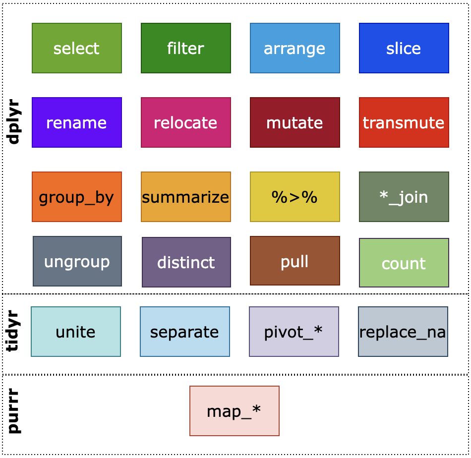
This section will cover the following:
-
select, for selecting or deselecting columns -
filter, for filtering rows -
arrange, for reordering rows -
slice, for selecting rows with criteria or by row numbers -
rename, for renaming attributes -
relocate, for adjusting the order of the columns -
mutateandtransmute, for adding new columns -
group_byandsummarize, for grouping rows together and summarizing information about the group
We will also discuss the |> operator to coordinate multiple actions seamlessly.
Be sure to bookmark the dplyr cheatsheet which will come in handy and useful for exploring more verbs available.
2.3.3 Selecting columns with select
The selection of attributes occurs when you want to focus on a subset of the attributes of a dataset at hand. The function select allows the selection in multiple possible ways.
In the simplest form of select, we list the attributes we wish to include in the data with a comma in between. For instance, we may only want to focus on the model name, miles per gallon, the number of cylinders, and the engine design.
select(mtcars_tibble, model_name, mpg, cyl, vs)## # A tibble: 32 × 4
## model_name mpg cyl vs
## <chr> <dbl> <dbl> <dbl>
## 1 Mazda RX4 21 6 0
## 2 Mazda RX4 Wag 21 6 0
## 3 Datsun 710 22.8 4 1
## 4 Hornet 4 Drive 21.4 6 1
## 5 Hornet Sportabout 18.7 8 0
## 6 Valiant 18.1 6 1
## 7 Duster 360 14.3 8 0
## 8 Merc 240D 24.4 4 1
## 9 Merc 230 22.8 4 1
## 10 Merc 280 19.2 6 1
## # ℹ 22 more rowsAlternatively, we may want the model name and all the columns that appear between mpg and wt.
select(mtcars_tibble, model_name, mpg:wt)## # A tibble: 32 × 7
## model_name mpg cyl disp hp drat wt
## <chr> <dbl> <dbl> <dbl> <dbl> <dbl> <dbl>
## 1 Mazda RX4 21 6 160 110 3.9 2.62
## 2 Mazda RX4 Wag 21 6 160 110 3.9 2.88
## 3 Datsun 710 22.8 4 108 93 3.85 2.32
## 4 Hornet 4 Drive 21.4 6 258 110 3.08 3.22
## 5 Hornet Sportabout 18.7 8 360 175 3.15 3.44
## 6 Valiant 18.1 6 225 105 2.76 3.46
## 7 Duster 360 14.3 8 360 245 3.21 3.57
## 8 Merc 240D 24.4 4 147. 62 3.69 3.19
## 9 Merc 230 22.8 4 141. 95 3.92 3.15
## 10 Merc 280 19.2 6 168. 123 3.92 3.44
## # ℹ 22 more rowsWe can also provide something more complex. select can receive attribute matching options like starts_with, ends_with, and contains. The following example demonstrates the use of some of these.
select(mtcars_tibble, cyl | !starts_with("m") & contains("a"))## # A tibble: 32 × 5
## cyl drat am gear carb
## <dbl> <dbl> <dbl> <dbl> <dbl>
## 1 6 3.9 1 4 4
## 2 6 3.9 1 4 4
## 3 4 3.85 1 4 1
## 4 6 3.08 0 3 1
## 5 8 3.15 0 3 2
## 6 6 2.76 0 3 1
## 7 8 3.21 0 3 4
## 8 4 3.69 0 4 2
## 9 4 3.92 0 4 2
## 10 6 3.92 0 4 4
## # ℹ 22 more rowsThe criterion for selection here: in addition tompg and cyl, any attribute whose name starts with some character other than “m” and contains “a” somewhere.
Going one step further, we can also supply a regular expression to do the matching. Recall that ^ and $ are the start and end of a string, respectively, and [a-z]{3,5} means any lowercase alphabet sequence having length between 3 and 5. Have a look at the following example.
## # A tibble: 32 × 7
## mpg cyl disp drat qsec gear carb
## <dbl> <dbl> <dbl> <dbl> <dbl> <dbl> <dbl>
## 1 21 6 160 3.9 16.5 4 4
## 2 21 6 160 3.9 17.0 4 4
## 3 22.8 4 108 3.85 18.6 4 1
## 4 21.4 6 258 3.08 19.4 3 1
## 5 18.7 8 360 3.15 17.0 3 2
## 6 18.1 6 225 2.76 20.2 3 1
## 7 14.3 8 360 3.21 15.8 3 4
## 8 24.4 4 147. 3.69 20 4 2
## 9 22.8 4 141. 3.92 22.9 4 2
## 10 19.2 6 168. 3.92 18.3 4 4
## # ℹ 22 more rowsThe regular expression here means return any columns that have “lowercase name with length between 3 and 5”.
2.3.4 Filtering rows with filter
Let us turn our attention now to the rows. The function filter allows us to select rows using some criteria. The syntax is to provide a Boolean expression for what should be included in the filtered dataset.
We can select all car models with 8 cylinders. Note how cyl == 8 is an expression that evalutes to either TRUE or FALSE depending on whether the attribute cyl of the row has a value of 8.
filter(mtcars_tibble, cyl == 8)## # A tibble: 14 × 12
## model_name mpg cyl disp hp drat wt qsec vs am gear carb
## <chr> <dbl> <dbl> <dbl> <dbl> <dbl> <dbl> <dbl> <dbl> <dbl> <dbl> <dbl>
## 1 Hornet Spo… 18.7 8 360 175 3.15 3.44 17.0 0 0 3 2
## 2 Duster 360 14.3 8 360 245 3.21 3.57 15.8 0 0 3 4
## 3 Merc 450SE 16.4 8 276. 180 3.07 4.07 17.4 0 0 3 3
## 4 Merc 450SL 17.3 8 276. 180 3.07 3.73 17.6 0 0 3 3
## 5 Merc 450SLC 15.2 8 276. 180 3.07 3.78 18 0 0 3 3
## 6 Cadillac F… 10.4 8 472 205 2.93 5.25 18.0 0 0 3 4
## 7 Lincoln Co… 10.4 8 460 215 3 5.42 17.8 0 0 3 4
## 8 Chrysler I… 14.7 8 440 230 3.23 5.34 17.4 0 0 3 4
## 9 Dodge Chal… 15.5 8 318 150 2.76 3.52 16.9 0 0 3 2
## 10 AMC Javelin 15.2 8 304 150 3.15 3.44 17.3 0 0 3 2
## 11 Camaro Z28 13.3 8 350 245 3.73 3.84 15.4 0 0 3 4
## 12 Pontiac Fi… 19.2 8 400 175 3.08 3.84 17.0 0 0 3 2
## 13 Ford Pante… 15.8 8 351 264 4.22 3.17 14.5 0 1 5 4
## 14 Maserati B… 15 8 301 335 3.54 3.57 14.6 0 1 5 8We could be more picky and refine our search by including more attributes to filter by.
filter(mtcars_tibble, cyl == 8, am == 1, hp > 300)## # A tibble: 1 × 12
## model_name mpg cyl disp hp drat wt qsec vs am gear carb
## <chr> <dbl> <dbl> <dbl> <dbl> <dbl> <dbl> <dbl> <dbl> <dbl> <dbl> <dbl>
## 1 Maserati Bo… 15 8 301 335 3.54 3.57 14.6 0 1 5 8Here, we requested a new tibble that contains rows with 8 cylinders, a manual transmission, and a gross horsepower over 300.
We may be interested in fetching a particular row in the dataset, say, the information associated with the car model “Datsun 710”. We can also use filter to achieve this task.
filter(mtcars_tibble, model_name == "Datsun 710")## # A tibble: 1 × 12
## model_name mpg cyl disp hp drat wt qsec vs am gear carb
## <chr> <dbl> <dbl> <dbl> <dbl> <dbl> <dbl> <dbl> <dbl> <dbl> <dbl> <dbl>
## 1 Datsun 710 22.8 4 108 93 3.85 2.32 18.6 1 1 4 1
2.3.5 Re-arranging rows with arrange
It may be necessary to rearrange the order of the rows to aid our understanding of the meaning of the dataset. The function arrange allows us to do just that.
To arrange rows, we state a list of attributes in the order we want to use for re-arranging. For instance, we can rearrange the rows by gross horsepower (hp).
arrange(mtcars_tibble, hp)## # A tibble: 32 × 12
## model_name mpg cyl disp hp drat wt qsec vs am gear carb
## <chr> <dbl> <dbl> <dbl> <dbl> <dbl> <dbl> <dbl> <dbl> <dbl> <dbl> <dbl>
## 1 Honda Civic 30.4 4 75.7 52 4.93 1.62 18.5 1 1 4 2
## 2 Merc 240D 24.4 4 147. 62 3.69 3.19 20 1 0 4 2
## 3 Toyota Cor… 33.9 4 71.1 65 4.22 1.84 19.9 1 1 4 1
## 4 Fiat 128 32.4 4 78.7 66 4.08 2.2 19.5 1 1 4 1
## 5 Fiat X1-9 27.3 4 79 66 4.08 1.94 18.9 1 1 4 1
## 6 Porsche 91… 26 4 120. 91 4.43 2.14 16.7 0 1 5 2
## 7 Datsun 710 22.8 4 108 93 3.85 2.32 18.6 1 1 4 1
## 8 Merc 230 22.8 4 141. 95 3.92 3.15 22.9 1 0 4 2
## 9 Toyota Cor… 21.5 4 120. 97 3.7 2.46 20.0 1 0 3 1
## 10 Valiant 18.1 6 225 105 2.76 3.46 20.2 1 0 3 1
## # ℹ 22 more rowsBy default, arrange will reorder in ascending order. If we wish to reorder in descending order, we put the attribute in a desc function call. While we are at it, let us break ties in hp and order by miles per gallon (mpg).
## # A tibble: 32 × 12
## model_name mpg cyl disp hp drat wt qsec vs am gear carb
## <chr> <dbl> <dbl> <dbl> <dbl> <dbl> <dbl> <dbl> <dbl> <dbl> <dbl> <dbl>
## 1 Maserati B… 15 8 301 335 3.54 3.57 14.6 0 1 5 8
## 2 Ford Pante… 15.8 8 351 264 4.22 3.17 14.5 0 1 5 4
## 3 Camaro Z28 13.3 8 350 245 3.73 3.84 15.4 0 0 3 4
## 4 Duster 360 14.3 8 360 245 3.21 3.57 15.8 0 0 3 4
## 5 Chrysler I… 14.7 8 440 230 3.23 5.34 17.4 0 0 3 4
## 6 Lincoln Co… 10.4 8 460 215 3 5.42 17.8 0 0 3 4
## 7 Cadillac F… 10.4 8 472 205 2.93 5.25 18.0 0 0 3 4
## 8 Merc 450SLC 15.2 8 276. 180 3.07 3.78 18 0 0 3 3
## 9 Merc 450SE 16.4 8 276. 180 3.07 4.07 17.4 0 0 3 3
## 10 Merc 450SL 17.3 8 276. 180 3.07 3.73 17.6 0 0 3 3
## # ℹ 22 more rows
2.3.6 Selecting rows with slice
The function is for selecting rows by specifying the rows position. You can specify one row with its row number, a range of rows with a number pair A:B where you can have an expression involving the function n to specify the number of rows in the data.
The following use of slice() uses the range (n()-10):(n()-2) is the range starting from the tenth row from the last and ending at the second to last row.
## # A tibble: 9 × 12
## model_name mpg cyl disp hp drat wt qsec vs am gear carb
## <chr> <dbl> <dbl> <dbl> <dbl> <dbl> <dbl> <dbl> <dbl> <dbl> <dbl> <dbl>
## 1 Dodge Chall… 15.5 8 318 150 2.76 3.52 16.9 0 0 3 2
## 2 AMC Javelin 15.2 8 304 150 3.15 3.44 17.3 0 0 3 2
## 3 Camaro Z28 13.3 8 350 245 3.73 3.84 15.4 0 0 3 4
## 4 Pontiac Fir… 19.2 8 400 175 3.08 3.84 17.0 0 0 3 2
## 5 Fiat X1-9 27.3 4 79 66 4.08 1.94 18.9 1 1 4 1
## 6 Porsche 914… 26 4 120. 91 4.43 2.14 16.7 0 1 5 2
## 7 Lotus Europa 30.4 4 95.1 113 3.77 1.51 16.9 1 1 5 2
## 8 Ford Panter… 15.8 8 351 264 4.22 3.17 14.5 0 1 5 4
## 9 Ferrari Dino 19.7 6 145 175 3.62 2.77 15.5 0 1 5 6We can also use slice_head(n = NUMBER) and slice_tail(n = NUMBER) to select the top NUMBER rows and the last NUMBER rows, respectively.
slice_head(mtcars_tibble, n = 2)## # A tibble: 2 × 12
## model_name mpg cyl disp hp drat wt qsec vs am gear carb
## <chr> <dbl> <dbl> <dbl> <dbl> <dbl> <dbl> <dbl> <dbl> <dbl> <dbl> <dbl>
## 1 Mazda RX4 21 6 160 110 3.9 2.62 16.5 0 1 4 4
## 2 Mazda RX4 W… 21 6 160 110 3.9 2.88 17.0 0 1 4 4
slice_tail(mtcars_tibble, n = 2)## # A tibble: 2 × 12
## model_name mpg cyl disp hp drat wt qsec vs am gear carb
## <chr> <dbl> <dbl> <dbl> <dbl> <dbl> <dbl> <dbl> <dbl> <dbl> <dbl> <dbl>
## 1 Maserati Bo… 15 8 301 335 3.54 3.57 14.6 0 1 5 8
## 2 Volvo 142E 21.4 4 121 109 4.11 2.78 18.6 1 1 4 2If we are interested in some particular row, we can use slice for that as well.
slice(mtcars_tibble, 3)## # A tibble: 1 × 12
## model_name mpg cyl disp hp drat wt qsec vs am gear carb
## <chr> <dbl> <dbl> <dbl> <dbl> <dbl> <dbl> <dbl> <dbl> <dbl> <dbl> <dbl>
## 1 Datsun 710 22.8 4 108 93 3.85 2.32 18.6 1 1 4 1We can also select a random row by using slice_sample. In this example, each row has an equal chance of being selected.
slice_sample(mtcars_tibble)## # A tibble: 1 × 12
## model_name mpg cyl disp hp drat wt qsec vs am gear carb
## <chr> <dbl> <dbl> <dbl> <dbl> <dbl> <dbl> <dbl> <dbl> <dbl> <dbl> <dbl>
## 1 Fiat X1-9 27.3 4 79 66 4.08 1.94 18.9 1 1 4 1
2.3.7 Renaming columns with rename
This function allows you to rename a specific column. The syntax is NEW_NAME = OLD_NAME. Below, we replace the name wt with weight amd cyl with cylinder.
rename(mtcars_tibble, weight = wt, cylinder = cyl)## # A tibble: 32 × 12
## model_name mpg cylinder disp hp drat weight qsec vs am gear
## <chr> <dbl> <dbl> <dbl> <dbl> <dbl> <dbl> <dbl> <dbl> <dbl> <dbl>
## 1 Mazda RX4 21 6 160 110 3.9 2.62 16.5 0 1 4
## 2 Mazda RX4 Wag 21 6 160 110 3.9 2.88 17.0 0 1 4
## 3 Datsun 710 22.8 4 108 93 3.85 2.32 18.6 1 1 4
## 4 Hornet 4 Dri… 21.4 6 258 110 3.08 3.22 19.4 1 0 3
## 5 Hornet Sport… 18.7 8 360 175 3.15 3.44 17.0 0 0 3
## 6 Valiant 18.1 6 225 105 2.76 3.46 20.2 1 0 3
## 7 Duster 360 14.3 8 360 245 3.21 3.57 15.8 0 0 3
## 8 Merc 240D 24.4 4 147. 62 3.69 3.19 20 1 0 4
## 9 Merc 230 22.8 4 141. 95 3.92 3.15 22.9 1 0 4
## 10 Merc 280 19.2 6 168. 123 3.92 3.44 18.3 1 0 4
## # ℹ 22 more rows
## # ℹ 1 more variable: carb <dbl>
2.3.8 Relocating column positions with relocate
Sometimes you may want to change the order of columns by moving a column from the present location to another. We can relocate a column using the relocate function by specifying which column should go where. The syntax is relocate(DATA_NAME,ATTRIBUTE,NEW_LOCATION).
The specification for the new location is either by .before=NAME or by .after=NAME, where NAME is the name of a column.
relocate(mtcars_tibble, am, .before = mpg)## # A tibble: 32 × 12
## model_name am mpg cyl disp hp drat wt qsec vs gear carb
## <chr> <dbl> <dbl> <dbl> <dbl> <dbl> <dbl> <dbl> <dbl> <dbl> <dbl> <dbl>
## 1 Mazda RX4 1 21 6 160 110 3.9 2.62 16.5 0 4 4
## 2 Mazda RX4 … 1 21 6 160 110 3.9 2.88 17.0 0 4 4
## 3 Datsun 710 1 22.8 4 108 93 3.85 2.32 18.6 1 4 1
## 4 Hornet 4 D… 0 21.4 6 258 110 3.08 3.22 19.4 1 3 1
## 5 Hornet Spo… 0 18.7 8 360 175 3.15 3.44 17.0 0 3 2
## 6 Valiant 0 18.1 6 225 105 2.76 3.46 20.2 1 3 1
## 7 Duster 360 0 14.3 8 360 245 3.21 3.57 15.8 0 3 4
## 8 Merc 240D 0 24.4 4 147. 62 3.69 3.19 20 1 4 2
## 9 Merc 230 0 22.8 4 141. 95 3.92 3.15 22.9 1 4 2
## 10 Merc 280 0 19.2 6 168. 123 3.92 3.44 18.3 1 4 4
## # ℹ 22 more rowsHere we moved the column am to the front, just before mpg.
2.3.9 Adding new columns using mutate
The function mutate can be used for modification or creation of a new column using some function of the values of existing columns. Let us see an example before getting into the details.
Suppose we are interested in calculating the ratio between the numbers of cylinders and forward gears for each car model. We can do this by appending a new column with the calculated ratios using mutate.
mtcars_with_ratio <- mutate(mtcars_tibble,
cyl_gear_ratio = cyl / gear)
mtcars_with_ratio## # A tibble: 32 × 13
## model_name mpg cyl disp hp drat wt qsec vs am gear carb
## <chr> <dbl> <dbl> <dbl> <dbl> <dbl> <dbl> <dbl> <dbl> <dbl> <dbl> <dbl>
## 1 Mazda RX4 21 6 160 110 3.9 2.62 16.5 0 1 4 4
## 2 Mazda RX4 … 21 6 160 110 3.9 2.88 17.0 0 1 4 4
## 3 Datsun 710 22.8 4 108 93 3.85 2.32 18.6 1 1 4 1
## 4 Hornet 4 D… 21.4 6 258 110 3.08 3.22 19.4 1 0 3 1
## 5 Hornet Spo… 18.7 8 360 175 3.15 3.44 17.0 0 0 3 2
## 6 Valiant 18.1 6 225 105 2.76 3.46 20.2 1 0 3 1
## 7 Duster 360 14.3 8 360 245 3.21 3.57 15.8 0 0 3 4
## 8 Merc 240D 24.4 4 147. 62 3.69 3.19 20 1 0 4 2
## 9 Merc 230 22.8 4 141. 95 3.92 3.15 22.9 1 0 4 2
## 10 Merc 280 19.2 6 168. 123 3.92 3.44 18.3 1 0 4 4
## # ℹ 22 more rows
## # ℹ 1 more variable: cyl_gear_ratio <dbl>Unfortunately, the new column appears at the very end which may not be desirable. We can fix this with the following adjustment.
mtcars_with_ratio <- mutate(mtcars_tibble,
cyl_gear_ratio = cyl / gear,
.before = mpg)
mtcars_with_ratio## # A tibble: 32 × 13
## model_name cyl_gear_ratio mpg cyl disp hp drat wt qsec vs
## <chr> <dbl> <dbl> <dbl> <dbl> <dbl> <dbl> <dbl> <dbl> <dbl>
## 1 Mazda RX4 1.5 21 6 160 110 3.9 2.62 16.5 0
## 2 Mazda RX4 Wag 1.5 21 6 160 110 3.9 2.88 17.0 0
## 3 Datsun 710 1 22.8 4 108 93 3.85 2.32 18.6 1
## 4 Hornet 4 Drive 2 21.4 6 258 110 3.08 3.22 19.4 1
## 5 Hornet Sporta… 2.67 18.7 8 360 175 3.15 3.44 17.0 0
## 6 Valiant 2 18.1 6 225 105 2.76 3.46 20.2 1
## 7 Duster 360 2.67 14.3 8 360 245 3.21 3.57 15.8 0
## 8 Merc 240D 1 24.4 4 147. 62 3.69 3.19 20 1
## 9 Merc 230 1 22.8 4 141. 95 3.92 3.15 22.9 1
## 10 Merc 280 1.5 19.2 6 168. 123 3.92 3.44 18.3 1
## # ℹ 22 more rows
## # ℹ 3 more variables: am <dbl>, gear <dbl>, carb <dbl>By specifying an additional .before argument with the value mpg, we inform dplyr that the new column cyl_gear_ratio should appear before the column mpg, which is the first column in the dataset.
Generally speaking, the syntax for mutate is:
mutate(DATA_SET_NAME, NEW_NAME = EXPRESSION, OPTION)
where:
- The
NEW_NAME = EXPRESSIONspecifies the name of the new attribute and how to compute it, andOPTIONis an option to specify the location of the new attribute relative to the existing attributes. - The position option is either of the form
.before=VALUEor of the form.after=VALUEwithVALUEspecifying the name of the column where the new column will appear before or after; it can also receive a number indicating the position for the newly inserted column.
- The
EXPRESSIONcan be either a mathematical expression or a function call.
Let us see another example. In addition to calculating the ratio from before, we will create another column containing the make of the car. We will do this by extracting the first word from model_name using a regular expression. Let us amend our mutate code from before to include the changes.
mtcars_mutated <- mutate(mtcars_tibble,
cyl_gear_ratio = cyl / gear,
make = str_replace(model_name, " .*", ""),
.before = mpg)
mtcars_mutated## # A tibble: 32 × 14
## model_name cyl_gear_ratio make mpg cyl disp hp drat wt qsec
## <chr> <dbl> <chr> <dbl> <dbl> <dbl> <dbl> <dbl> <dbl> <dbl>
## 1 Mazda RX4 1.5 Mazda 21 6 160 110 3.9 2.62 16.5
## 2 Mazda RX4 Wag 1.5 Mazda 21 6 160 110 3.9 2.88 17.0
## 3 Datsun 710 1 Dats… 22.8 4 108 93 3.85 2.32 18.6
## 4 Hornet 4 Drive 2 Horn… 21.4 6 258 110 3.08 3.22 19.4
## 5 Hornet Sporta… 2.67 Horn… 18.7 8 360 175 3.15 3.44 17.0
## 6 Valiant 2 Vali… 18.1 6 225 105 2.76 3.46 20.2
## 7 Duster 360 2.67 Dust… 14.3 8 360 245 3.21 3.57 15.8
## 8 Merc 240D 1 Merc 24.4 4 147. 62 3.69 3.19 20
## 9 Merc 230 1 Merc 22.8 4 141. 95 3.92 3.15 22.9
## 10 Merc 280 1.5 Merc 19.2 6 168. 123 3.92 3.44 18.3
## # ℹ 22 more rows
## # ℹ 4 more variables: vs <dbl>, am <dbl>, gear <dbl>, carb <dbl>To form the make column, we use the function str_replace; we look for substrings that match the pattern " .*" (one white space and then any number of characters following it) and replace it with an empty string "", leaving only the first word, as desired. String operations are applicable to strings, which is what appears in the column make.
Note that the original dataset, before mutation, remains unchanged in mtcars_tibble.
mtcars_tibble## # A tibble: 32 × 12
## model_name mpg cyl disp hp drat wt qsec vs am gear carb
## <chr> <dbl> <dbl> <dbl> <dbl> <dbl> <dbl> <dbl> <dbl> <dbl> <dbl> <dbl>
## 1 Mazda RX4 21 6 160 110 3.9 2.62 16.5 0 1 4 4
## 2 Mazda RX4 … 21 6 160 110 3.9 2.88 17.0 0 1 4 4
## 3 Datsun 710 22.8 4 108 93 3.85 2.32 18.6 1 1 4 1
## 4 Hornet 4 D… 21.4 6 258 110 3.08 3.22 19.4 1 0 3 1
## 5 Hornet Spo… 18.7 8 360 175 3.15 3.44 17.0 0 0 3 2
## 6 Valiant 18.1 6 225 105 2.76 3.46 20.2 1 0 3 1
## 7 Duster 360 14.3 8 360 245 3.21 3.57 15.8 0 0 3 4
## 8 Merc 240D 24.4 4 147. 62 3.69 3.19 20 1 0 4 2
## 9 Merc 230 22.8 4 141. 95 3.92 3.15 22.9 1 0 4 2
## 10 Merc 280 19.2 6 168. 123 3.92 3.44 18.3 1 0 4 4
## # ℹ 22 more rowsHow many different makes are there? We can use unique for removing duplicates to find out.
## [1] "Mazda" "Datsun" "Hornet" "Valiant" "Duster" "Merc"
## [7] "Cadillac" "Lincoln" "Chrysler" "Fiat" "Honda" "Toyota"
## [13] "Dodge" "AMC" "Camaro" "Pontiac" "Porsche" "Lotus"
## [19] "Ford" "Ferrari" "Maserati" "Volvo"When an existing column is given in the specification, no new column is created and the existing column is modified instead. For instance, the following rounds wt to the nearest integer value.
## # A tibble: 32 × 12
## model_name mpg cyl disp hp drat wt qsec vs am gear carb
## <chr> <dbl> <dbl> <dbl> <dbl> <dbl> <dbl> <dbl> <dbl> <dbl> <dbl> <dbl>
## 1 Mazda RX4 21 6 160 110 3.9 3 16.5 0 1 4 4
## 2 Mazda RX4 … 21 6 160 110 3.9 3 17.0 0 1 4 4
## 3 Datsun 710 22.8 4 108 93 3.85 2 18.6 1 1 4 1
## 4 Hornet 4 D… 21.4 6 258 110 3.08 3 19.4 1 0 3 1
## 5 Hornet Spo… 18.7 8 360 175 3.15 3 17.0 0 0 3 2
## 6 Valiant 18.1 6 225 105 2.76 3 20.2 1 0 3 1
## 7 Duster 360 14.3 8 360 245 3.21 4 15.8 0 0 3 4
## 8 Merc 240D 24.4 4 147. 62 3.69 3 20 1 0 4 2
## 9 Merc 230 22.8 4 141. 95 3.92 3 22.9 1 0 4 2
## 10 Merc 280 19.2 6 168. 123 3.92 3 18.3 1 0 4 4
## # ℹ 22 more rowsWe can also modify multiple columns in a single pass, say, wt, mpg, and qsec should all be rounded to the nearest integer. We can accomplish this using a combination of mutate with the helper dplyr verb across.
## # A tibble: 32 × 12
## model_name mpg cyl disp hp drat wt qsec vs am gear carb
## <chr> <dbl> <dbl> <dbl> <dbl> <dbl> <dbl> <dbl> <dbl> <dbl> <dbl> <dbl>
## 1 Mazda RX4 21 6 160 110 3.9 3 16 0 1 4 4
## 2 Mazda RX4 … 21 6 160 110 3.9 3 17 0 1 4 4
## 3 Datsun 710 23 4 108 93 3.85 2 19 1 1 4 1
## 4 Hornet 4 D… 21 6 258 110 3.08 3 19 1 0 3 1
## 5 Hornet Spo… 19 8 360 175 3.15 3 17 0 0 3 2
## 6 Valiant 18 6 225 105 2.76 3 20 1 0 3 1
## 7 Duster 360 14 8 360 245 3.21 4 16 0 0 3 4
## 8 Merc 240D 24 4 147. 62 3.69 3 20 1 0 4 2
## 9 Merc 230 23 4 141. 95 3.92 3 23 1 0 4 2
## 10 Merc 280 19 6 168. 123 3.92 3 18 1 0 4 4
## # ℹ 22 more rows
2.3.10 The function transmute
The function transmute is a variant of mutate where we keep only the new columns generated.
only_the_new_stuff <- transmute(mtcars_tibble,
cyl_gear_ratio = cyl / gear,
make = str_replace(model_name, " .*", ""))
only_the_new_stuff## # A tibble: 32 × 2
## cyl_gear_ratio make
## <dbl> <chr>
## 1 1.5 Mazda
## 2 1.5 Mazda
## 3 1 Datsun
## 4 2 Hornet
## 5 2.67 Hornet
## 6 2 Valiant
## 7 2.67 Duster
## 8 1 Merc
## 9 1 Merc
## 10 1.5 Merc
## # ℹ 22 more rows
2.3.11 The pair group_by and summarize
Suppose you are interested in exploring the relationship between the number of cylinders in a car model and the miles per gallon it has. One way to examine this is to look at some summary statistic, say the average, of the miles per gallon for car models with 6 cylinders, car models with 7 cylinders, and car models with 8 cylinders.
When thinking about the problem in this way, we have effectively divided up all of the rows in the dataset into three groups, where the group a car model will belong to is determined by the number of cylinders it has.
dplyr accomplishes this using the function group_by(). The syntax for group_by() is simple: simply list the attributes with which you want to build groups. Let us give an example on how to use it.
grouped_by_cl <- group_by(mtcars_tibble, cyl)
slice_head(grouped_by_cl, n=2) # show 2 rows per group## # A tibble: 6 × 12
## # Groups: cyl [3]
## model_name mpg cyl disp hp drat wt qsec vs am gear carb
## <chr> <dbl> <dbl> <dbl> <dbl> <dbl> <dbl> <dbl> <dbl> <dbl> <dbl> <dbl>
## 1 Datsun 710 22.8 4 108 93 3.85 2.32 18.6 1 1 4 1
## 2 Merc 240D 24.4 4 147. 62 3.69 3.19 20 1 0 4 2
## 3 Mazda RX4 21 6 160 110 3.9 2.62 16.5 0 1 4 4
## 4 Mazda RX4 W… 21 6 160 110 3.9 2.88 17.0 0 1 4 4
## 5 Hornet Spor… 18.7 8 360 175 3.15 3.44 17.0 0 0 3 2
## 6 Duster 360 14.3 8 360 245 3.21 3.57 15.8 0 0 3 4We can spot two rows shown per each cyl group. group_by() alone is often not useful. To make something out of this, we need to summarize some piece of information using these groups, e.g. the average mpg per group as is needed for our task.
The summary function is called summarize(). Let us amend our above grouping code to include the summary.
grouped_by_cl <- group_by(mtcars_tibble, cyl)
summarized <- summarize(grouped_by_cl,
count = n(),
avg_mpg = mean(mpg))
summarized## # A tibble: 3 × 3
## cyl count avg_mpg
## <dbl> <int> <dbl>
## 1 4 11 26.7
## 2 6 7 19.7
## 3 8 14 15.1This table looks more like what we would expect. Our summary calculates two summaries, each reflected in a column in the above table:
-
count, the number of car models belonging to the group -
avg_mpg, the average miles per gallon of car models in the group
The summary results make sense. More cylinders translates to more power, but it also means more moving parts which can hurt efficiency. Therefore, it seems an association exists where the more cylinders a car has, the lower its miles per gallon.
These functions come handy when you want to examine data by grouping rows and summarize some information with respect to each group.
2.3.12 Coordinating multiple actions using |>
Let us revise a bit our previous study. Curious about the joint effect of the numbers of cylinders and the transmission of the car, you decide to group by both cyl and am. After summarizing the groups, you calculate the counts in each group and the average mpg. Finally, after the summary is done, you would like to remove any groups from the summary that have less than 2 cars.
Your analysis pipeline, then, would be composed of three steps:
cyl and am, the number of cylinders.2. Summarize to calculate the average miles per gallon per group.
3. Filter out rows that are below the average miles per gallon.
A first solution for this task might look like the following.
# step 1
grouped_by_cl <- group_by(mtcars_tibble, cyl, am)
# step 2
summarized <- summarize(grouped_by_cl,
count = n(),
avg_mpg = mean(mpg))
# step 3
avg_mpg_counts <- filter(summarized, count > 2)
avg_mpg_counts## # A tibble: 5 × 4
## # Groups: cyl [3]
## cyl am count avg_mpg
## <dbl> <dbl> <int> <dbl>
## 1 4 0 3 22.9
## 2 4 1 8 28.1
## 3 6 0 4 19.1
## 4 6 1 3 20.6
## 5 8 0 12 15.0Observe how the code we have just written is quite cumbersome. It introduces several intermediate products that we do not need, namely, the names grouped_by_cl and summarized. It can also be difficult to come up with descriptive names.
Conveniently, there is a construct from base R called the “pipe” which allows us to pass the results from one function as input to another. The way to use piping is simple.
- You start by stating the initial dataset.
- For each operation to form, you append
|>and then the operation, where you omit the dataset name part. - If you need to save the result in a data set, you use the assignment operator
<-at the beginning as usual.
Thus, we can rewrite our first solution as follows.
avg_mpg_counts <- mtcars |>
group_by(cyl, am) |>
summarize(count = n(),
avg_mpg = mean(mpg)) |>
filter(count > 2)This solution is much easier to read than our first; we can clearly identify the transformations being performed on the data. It is good to read |> as “then”.
Note that there is not much mystery with |>. All the pipe operator does is place an object into the first argument of a function. So, when we say mtcars |> group_by(cyl, am), the pipe changes this to group_by(mtcars, cyl, am). Or, more generally, if we have x |> func(y), this is changed to func(x, y).
Here is another use of the pipe, using our mtcars_mutated tibble from earlier.
## [1] "Mazda" "Datsun" "Hornet" "Valiant" "Duster" "Merc"
## [7] "Cadillac" "Lincoln" "Chrysler" "Fiat" "Honda" "Toyota"
## [13] "Dodge" "AMC" "Camaro" "Pontiac" "Porsche" "Lotus"
## [19] "Ford" "Ferrari" "Maserati" "Volvo"Neat! This one demonstrates some of the usefulness of pull over the traditional $ for accessing column data.
2.3.13 Practice makes perfect!
This section has covered a lot of dplyr functions for transforming datasets and, despite our best efforts, understanding what these functions are doing can quickly become overwhelming. The only way to truly understand these functions – and which ones should be used when confronted with a situation – is to practice using them.
Begin with the mtcars dataset from this section and run through each of the functions and the examples discussed here on your own. Observe what the dataset looks like before and after the transformation and try to understand what the transformation is.
Once you develop enough familiarity with these functions, try making small changes to our examples and coming up with your own transformations to apply. Be sure to include the |> operator whenever possible.
You may also wish to look at some of the datasets available to you when running the command data().
2.4 Tidy Transformations
In this section we turn to transformation techniques that are essential for achieving tidy data.
2.4.2 Uniting and separating columns
The third tidy data guideline states that each value must have its own cell. Sometimes this value may be split across multiple columns or merged in a single column.
In the case of the Miami bakery example, we saw that when the bakery records sale forecasts, the lower and upper bounds of the range are fused in a single cell. This makes extraction and analysis of these values difficult, especially when R treats the forecast column as a character sequence.
forecast_sales <- tibble(
week = c(1, 2, 3),
forecast = c("200-300", "300-400", "200-500")
)
forecast_sales## # A tibble: 3 × 2
## week forecast
## <dbl> <chr>
## 1 1 200-300
## 2 2 300-400
## 3 3 200-500A solution would be to split forecast into multiple columns, one giving the lower bound and the other the upper bound. The tidyr function separate accomplishes the work.
## # A tibble: 3 × 3
## week low high
## <dbl> <int> <int>
## 1 1 200 300
## 2 2 300 400
## 3 3 200 500We separate the columns based on the presence of the "-" character. The convert argument is set so that the lower and upper values can be treated as proper integers.
The tibble table5 displays the number of TB cases documented by the World Health Organization in Afghanistan, Brazil, and China between 1999 and 2000. The “year”, however, is a single value that has been split across a century and year column.
table5## # A tibble: 6 × 4
## country century year rate
## <chr> <chr> <chr> <chr>
## 1 Afghanistan 19 99 745/19987071
## 2 Afghanistan 20 00 2666/20595360
## 3 Brazil 19 99 37737/172006362
## 4 Brazil 20 00 80488/174504898
## 5 China 19 99 212258/1272915272
## 6 China 20 00 213766/1280428583The unite function can be used to merge a split value. Its functionality is similar to separate.
table5 |>
unite("year", century:year, sep="")## # A tibble: 6 × 3
## country year rate
## <chr> <chr> <chr>
## 1 Afghanistan 1999 745/19987071
## 2 Afghanistan 2000 2666/20595360
## 3 Brazil 1999 37737/172006362
## 4 Brazil 2000 80488/174504898
## 5 China 1999 212258/1272915272
## 6 China 2000 213766/1280428583We specify an empty string ("") in the sep argument to indicate no character delimiter should be used when merging the values.
Note also that the rate column needs tidying. We leave the tidying of this column as an exercise for the reader.
2.4.3 Pulling data from multiple sources
The fourth principle of tidy data stated that an observational unit should form a table. However, often times the observational unit we are measuring is split across multiple tables.
Let us suppose we are measuring student assessments in a class. The data is given to us in the form of two tables, one for exams and the other for assignments. We load the scores into our R environment with tibble.
exams <- tibble(name = c("Adriana", "Beth", "Candy", "Emily"),
midterm = c(90, 80, 95, 87),
final = c(99, 50, 70, 78))
assignments <- tibble(name = c("Adriana", "Beth", "Candy", "Florence"),
assign1 = c(80, 88, 93, 88),
assign2 = c(91, 61, 73, 83))
exams## # A tibble: 4 × 3
## name midterm final
## <chr> <dbl> <dbl>
## 1 Adriana 90 99
## 2 Beth 80 50
## 3 Candy 95 70
## 4 Emily 87 78
assignments## # A tibble: 4 × 3
## name assign1 assign2
## <chr> <dbl> <dbl>
## 1 Adriana 80 91
## 2 Beth 88 61
## 3 Candy 93 73
## 4 Florence 88 83If the observational unit is an assessment result, then some assessments are in one table and some assessments are in another. Therefore, according to this definition, the current arrangement of the data is not tidy. The data should be kept together in a single table.
You can combine two tibbles using a common attribute as the key for combining; that is, finding values appearing in both tibbles and then connecting rows having the names in common. In general, if there are multiple matches between the two tibbles concerning the attribute, each possible row matches will appear.
The construct for stitching together two tibbles together in this manner is called the join. The general syntax is:
JOIN_METHOD_NAME(DATA1, DATA2, by="NAME").
Here DATA1 and DATA2 are the names of the tibbles and NAME is the name of the key attributes. There are four types of join functions. The differences among them are in how they treat non-matching values.
-
left_join: Exclude any rows inDATA2with no matching values inDATA1. -
right_join; Exclude any rows inDATA1with no matching values inDATA2. -
inner_join: Exclude any rows inDATA2andDATA1with no matching values in the other data frame. -
full_join: No exclusions.
The example below shows the results of four join operations.
scores_left <- left_join(assignments, exams, by="name")
scores_left## # A tibble: 4 × 5
## name assign1 assign2 midterm final
## <chr> <dbl> <dbl> <dbl> <dbl>
## 1 Adriana 80 91 90 99
## 2 Beth 88 61 80 50
## 3 Candy 93 73 95 70
## 4 Florence 88 83 NA NA
scores_right <- right_join(assignments, exams, by="name")
scores_right## # A tibble: 4 × 5
## name assign1 assign2 midterm final
## <chr> <dbl> <dbl> <dbl> <dbl>
## 1 Adriana 80 91 90 99
## 2 Beth 88 61 80 50
## 3 Candy 93 73 95 70
## 4 Emily NA NA 87 78
scores_inner <- inner_join(assignments, exams, by = "name")
scores_inner## # A tibble: 3 × 5
## name assign1 assign2 midterm final
## <chr> <dbl> <dbl> <dbl> <dbl>
## 1 Adriana 80 91 90 99
## 2 Beth 88 61 80 50
## 3 Candy 93 73 95 70
scores_full <- full_join(assignments, exams, by="name")
scores_full## # A tibble: 5 × 5
## name assign1 assign2 midterm final
## <chr> <dbl> <dbl> <dbl> <dbl>
## 1 Adriana 80 91 90 99
## 2 Beth 88 61 80 50
## 3 Candy 93 73 95 70
## 4 Florence 88 83 NA NA
## 5 Emily NA NA 87 78The results of the join reveal some anomalies in our data. Namely, we see that Emily does not have any assignment scores nor does Florence have any exam scores. Hence, in the left, right, and full joins, we see values labeled NA appear where they would have those values. We call these missing values, which can be thought of as “holes” in the data. We will return to missing values in a later section.
An alternative to the join is to stack up the rows using bind_rows.
bind_rows(assignments, exams)## # A tibble: 8 × 5
## name assign1 assign2 midterm final
## <chr> <dbl> <dbl> <dbl> <dbl>
## 1 Adriana 80 91 NA NA
## 2 Beth 88 61 NA NA
## 3 Candy 93 73 NA NA
## 4 Florence 88 83 NA NA
## 5 Adriana NA NA 90 99
## 6 Beth NA NA 80 50
## 7 Candy NA NA 95 70
## 8 Emily NA NA 87 78Observe how this one does not join values where possible, and so there is redundancy in the rows that appear, e.g., Adriana appears twice. As a result, many missing values appear in the resulting table.
2.4.4 Pivoting
Let us return to the resulting table after the inner join.
scores_inner## # A tibble: 3 × 5
## name assign1 assign2 midterm final
## <chr> <dbl> <dbl> <dbl> <dbl>
## 1 Adriana 80 91 90 99
## 2 Beth 88 61 80 50
## 3 Candy 93 73 95 70The third property of tidy data is fulfilled now that the observational unit forms a single table. However, the joined table is still messy. The grades are split across four different columns and, therefore, multiple observations occur at each row.
To remedy this, we use pivot and, in terms of R, the function pivot_longer from the tidyr package. The syntax for pivot_longer can be complex, and so we do not go over it in detail. Here is how we can use it.
scores_long <- scores_inner |>
pivot_longer(c(assign1, assign2, midterm, final),
names_to = "assessment", values_to = "score")
scores_long## # A tibble: 12 × 3
## name assessment score
## <chr> <chr> <dbl>
## 1 Adriana assign1 80
## 2 Adriana assign2 91
## 3 Adriana midterm 90
## 4 Adriana final 99
## 5 Beth assign1 88
## 6 Beth assign2 61
## 7 Beth midterm 80
## 8 Beth final 50
## 9 Candy assign1 93
## 10 Candy assign2 73
## 11 Candy midterm 95
## 12 Candy final 70The usage above takes scores_inner, merges all the assessment columns, creates a new column with name assessment, and presents the corresponding values under the column score. Graphically, this is what a pivot longer transformation computes.
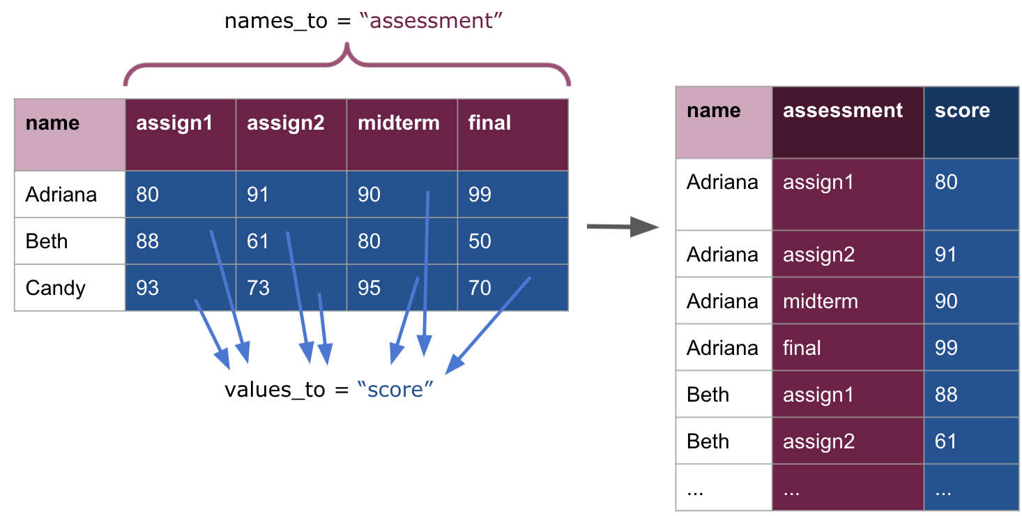
Observe how we can easily read off the three variables from this table: name, assessment, and score. We can be confident in knowing that this is tidy data.
If we wish to go in the other direction, we can use pivot_wider. The function pivot_wider grabs a pair of columns and spreads the pair into a series of columns. One column of the pair serves as the source for the new column names after spreading. For each value appearing in the source column, the function creates a new column by the name. The value appearing opposite to the source value appears as the value for the column corresponding to the source.
scores_long |>
pivot_wider(names_from = assessment, values_from = score)## # A tibble: 3 × 5
## name assign1 assign2 midterm final
## <chr> <dbl> <dbl> <dbl> <dbl>
## 1 Adriana 80 91 90 99
## 2 Beth 88 61 80 50
## 3 Candy 93 73 95 70Here is a visual demonstrating the pivot wider transformation:
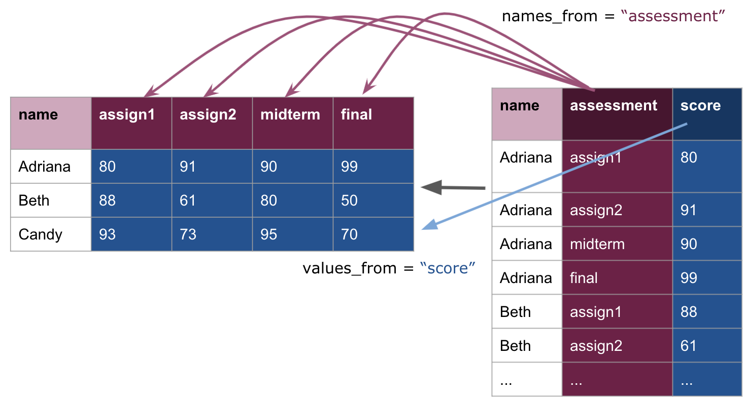
Note how this simply undoes what we have done, returning us to the original scores_inner table. We can also prefix each of the new columns with assess_.
scores_long |>
pivot_wider(names_from = assessment,
values_from = score, names_prefix = "assess_")## # A tibble: 3 × 5
## name assess_assign1 assess_assign2 assess_midterm assess_final
## <chr> <dbl> <dbl> <dbl> <dbl>
## 1 Adriana 80 91 90 99
## 2 Beth 88 61 80 50
## 3 Candy 93 73 95 70There are two details to note when working with the pivot functions.
-
pivot_widershould not be thought of as an “undo” operation. Likepivot_longerits primary purpose is also to make data tidy. Consider the following table and observe how each observation is scattered across two rows. The appropriate means to bring this data into tidiness is through an application ofpivot_wider.slice_head(table2, n = 5)## # A tibble: 5 × 4 ## country year type count ## <chr> <dbl> <chr> <dbl> ## 1 Afghanistan 1999 cases 745 ## 2 Afghanistan 1999 population 19987071 ## 3 Afghanistan 2000 cases 2666 ## 4 Afghanistan 2000 population 20595360 ## 5 Brazil 1999 cases 37737 -
pivot_longerandpivot_widerare not perfectly symmetrical operations. That is, there are cases where applyingpivot_wider, followed bypivot_longer, will not reproduce the exact same dataset. Consider such an application on the following dataset. Keep in mind the column names and how the column data types change at each pivot step.
2.5 Applying Functions to Columns
Situations can arise where we need to apply some function to a column. In this section we learn how to apply functions to columns using a construct called the map.
2.5.1 Prerequisites
As before, let us load tidyverse.
We will use the mtcars tibble again in this section so let us prepare the tibble by migrating the row names to a dedicated column. Note how the pipe operator can be used to help with the work.
mtcars_tibble <- mtcars |>
rownames_to_column("model_name")
2.5.2 What is a function anyway?
We have used several times by now the word “function”. Here are some basic rules about functions.
- A function is a block of code with a name that allows execution from other codes. This mean that you can take any part of a working block of code (i.e., all parentheses and brackets in the part have matching counterparts in the same part) and specify it to be a function.
- If the function is active in the present run of R, each time a code call the function, the code of the function runs. This means that R suspends the execution of the present code and processes the execution of the code of the function. When it finishes running the code of the function, it returns to the execution of the one it has suspended.
-
A function may take upon the role of computing a value. You can design a function so that it uses a special function
returnat the end so as to specify the value it has computed. Note that the use ofreturnis optional and, by default, R returns the last line of computation performed in the function. - If a function has the role of returning a value, the call itself represents the value it computes. So you store the value the function computes in a variable using an assignment.
- A function may require some number of values to use in its calculation. We call them arguments. When using a function that requires arguments, the arguments must appear in the call.
2.5.3 A very simple function
Here is a very simple function, one_to_ten, which prints the sequence of integers from 1 to 10. The definition of the function takes the form one_ten <- function() { ... }.
one_to_ten <- function() {
print(1:10)
}Here is what happens when you call the function.
one_to_ten()## [1] 1 2 3 4 5 6 7 8 9 10Note that the call stands alone, i.e., you can use it without anything else but its name and a pair of parentheses. By replacing the code appearing inside the curly brackets, you can define a different function with the same name one_to_ten.
Let us reverse the order in which the numbers appear.
one_to_ten <- function() {
print(10:1)
}Here is what happens when you call the function.
one_to_ten()## [1] 10 9 8 7 6 5 4 3 2 1The new behavior of one_to_ten substitutes the old one, and you cannot replay the behavior of the previous version (until, of course, you modify the function again).
2.5.4 Functions that compute a value
To make a function compute a value, you add a line return(VALUE) at the end of the code in the brackets. The function my_family returns a list of names for persons.
Remember the c function? The function creates a vector with 19 names as strings and returns the vector.
my_family <- function() {
c("Amy", "Billie", "Casey", "Debbie", "Eddie", "Freddie", "Gary",
"Hary", "Ivy", "Jackie", "Lily", "Mikey", "Nellie", "Odie",
"Paulie", "Quincy", "Ruby", "Stacey", "Tiffany")
}The call for the function produces the list that the function returns.
a <- my_family()
a## [1] "Amy" "Billie" "Casey" "Debbie" "Eddie" "Freddie" "Gary"
## [8] "Hary" "Ivy" "Jackie" "Lily" "Mikey" "Nellie" "Odie"
## [15] "Paulie" "Quincy" "Ruby" "Stacey" "Tiffany"Now whenever you need the 19-name list, you can either call the function or refer to the variable a that holds the list.
2.5.5 Functions that take arguments
To write a function that takes arguments, you determine how many arguments you need and determine the names you want to use for the arguments during the execution of the code for the function.
The function declaration now has the names of the arguments. You put them in the order you want to use with a comma in between. Below, we define a function that computes the max between 100 and the argument received. The function returns the argument so long as it is larger than 100.
passes_100 <- function(x) {
max(100, x)
}Here is a demonstration of how the function works.
passes_100(50) # a value smaller than 100## [1] 100
passes_100(2021) # a value larger than 100## [1] 2021
2.5.6 Applying functions using mutate
Let us now return to the discussion of how we can apply functions to a column. The meaning of apply is particular. What we mean by this is that we wish to run some function (which can receive an argument and return a value) to each row of a column. This can be useful if, say, some column is given in the wrong units or if the values in a column should be “cut off” at some threshold point.
Recall the tidied tibble mtcars_tibble.
mtcars_tibble## # A tibble: 32 × 11
## mpg cyl disp hp drat wt qsec vs am gear carb
## <dbl> <dbl> <dbl> <dbl> <dbl> <dbl> <dbl> <dbl> <dbl> <dbl> <dbl>
## 1 21 6 160 110 3.9 2.62 16.5 0 1 4 4
## 2 21 6 160 110 3.9 2.88 17.0 0 1 4 4
## 3 22.8 4 108 93 3.85 2.32 18.6 1 1 4 1
## 4 21.4 6 258 110 3.08 3.22 19.4 1 0 3 1
## 5 18.7 8 360 175 3.15 3.44 17.0 0 0 3 2
## 6 18.1 6 225 105 2.76 3.46 20.2 1 0 3 1
## 7 14.3 8 360 245 3.21 3.57 15.8 0 0 3 4
## 8 24.4 4 147. 62 3.69 3.19 20 1 0 4 2
## 9 22.8 4 141. 95 3.92 3.15 22.9 1 0 4 2
## 10 19.2 6 168. 123 3.92 3.44 18.3 1 0 4 4
## # ℹ 22 more rowsWe can spot two areas that require transformation:
- Convert the
wtcolumn from pounds to kilograms. - Cut off the values in
displso that no car model has a value larger than400.
We can address the first one by writing a function that multiples each value in the argument received by the conversion factor for kilograms. Let us test it out first with a simple vector.
wt_conversion <- function(x) {
x * 0.454
}
wt_conversion(100:105)## [1] 45.400 45.854 46.308 46.762 47.216 47.670To incorporate this into the tibble, we make a call to mutate using our function wt_conversion, which modifies the column wt.
mtcars_transformed <- mtcars_tibble |>
mutate(wt = wt_conversion(wt))
mtcars_transformed## # A tibble: 32 × 11
## mpg cyl disp hp drat wt qsec vs am gear carb
## <dbl> <dbl> <dbl> <dbl> <dbl> <dbl> <dbl> <dbl> <dbl> <dbl> <dbl>
## 1 21 6 160 110 3.9 1.19 16.5 0 1 4 4
## 2 21 6 160 110 3.9 1.31 17.0 0 1 4 4
## 3 22.8 4 108 93 3.85 1.05 18.6 1 1 4 1
## 4 21.4 6 258 110 3.08 1.46 19.4 1 0 3 1
## 5 18.7 8 360 175 3.15 1.56 17.0 0 0 3 2
## 6 18.1 6 225 105 2.76 1.57 20.2 1 0 3 1
## 7 14.3 8 360 245 3.21 1.62 15.8 0 0 3 4
## 8 24.4 4 147. 62 3.69 1.45 20 1 0 4 2
## 9 22.8 4 141. 95 3.92 1.43 22.9 1 0 4 2
## 10 19.2 6 168. 123 3.92 1.56 18.3 1 0 4 4
## # ℹ 22 more rowsWe have successfully applied a function we wrote to a column in a tibble!
The second task is peculiar. As with the first example, we can define a function that computes the minimum between the argument and the value 400.
cutoff_400 <- function(x) {
min(400, x)
}We could then apply the function to the column disp using a similar approach.
mtcars_transformed <- mtcars_tibble |>
mutate(disp = cutoff_400(disp))
mtcars_transformed## # A tibble: 32 × 11
## mpg cyl disp hp drat wt qsec vs am gear carb
## <dbl> <dbl> <dbl> <dbl> <dbl> <dbl> <dbl> <dbl> <dbl> <dbl> <dbl>
## 1 21 6 71.1 110 3.9 2.62 16.5 0 1 4 4
## 2 21 6 71.1 110 3.9 2.88 17.0 0 1 4 4
## 3 22.8 4 71.1 93 3.85 2.32 18.6 1 1 4 1
## 4 21.4 6 71.1 110 3.08 3.22 19.4 1 0 3 1
## 5 18.7 8 71.1 175 3.15 3.44 17.0 0 0 3 2
## 6 18.1 6 71.1 105 2.76 3.46 20.2 1 0 3 1
## 7 14.3 8 71.1 245 3.21 3.57 15.8 0 0 3 4
## 8 24.4 4 71.1 62 3.69 3.19 20 1 0 4 2
## 9 22.8 4 71.1 95 3.92 3.15 22.9 1 0 4 2
## 10 19.2 6 71.1 123 3.92 3.44 18.3 1 0 4 4
## # ℹ 22 more rowsThat didn’t work out so well. The new disp column contains the same value 71.1 for every row in the tibble! Did dplyr make a mistake? Is the function we wrote just totally wrong?
The error, actually, is not in anything we wrote per se, but in how R processes the function cutoff_400 during the mutate call. We expect to pass one number to the function cutoff_400 so that we can compare it against 400, but our function instead receives a vector of values when used inside a mutate verb. That is, the entire disp column of values is passed as an argument to the function cutoff_400.
While this was no problem for the wt_conversion function, cutoff_400 is not capable of handling a vector as an argument and returning a vector back.
To clarify the point, compare the result of these two functions after receiving the vector 399:405.
wt_conversion(399:405)## [1] 181.146 181.600 182.054 182.508 182.962 183.416 183.870
cutoff_400(399:405)## [1] 399wt_conversion performs an element-wise operation to each element of the sequence and, therefore, the first example works as intended. In the second, cutoff_400 computes the minimum of the vector (399) and returns the result of just that computation; no element-wise comparison is made.
To make cutoff_400 work as intended, we turn to a new programming construct called the map, prepared by the package purrr.
2.5.7 purrr maps
The main construct we will be using from purrr is called the map. A map applies a function, say the cutoff_400 function we just wrote, to each element of a vector or list.
purrr offers many flavors of map, depending on what the output vector should look like:
-
map_lgl()outputs a logical vector. -
map_int()outputs an integer vector. -
map_dbl()outputs a double vector. -
map_chr()outputs a character vector. -
map()outputs a list.
Here are some more examples of using map. Let us apply the wt_conversion to an input vector containing a sequence of values from 399 to 405.
map_dbl(399:405, wt_conversion)## [1] 181.146 181.600 182.054 182.508 182.962 183.416 183.870Observe how this resulting vector is the same one we obtained when applying wt_conversion without a map.
We can also define functions and pass it in on the spot. We call these anonymous functions. The following is an identity function: it simply outputs what it takes in.
map_int(1:5, function(x) x)## [1] 1 2 3 4 5A catch here is that the code after the comma, i.e.,
function(x) xspecifies in place the function to apply to each element of the series preceding the comma1:5. The function in questionfunction(x) xspecifies that the function will receive a value namedxand returns the value ofxwithout modification. Thus we call it an identity function. The external functionmap_intstates that the result of applying the identify function thus specified withfunction(x) xto each element of the sequence1:5will be presented as an integer.
We could write the above anonymous function more compactly.
map_int(1:5, \(x) x)## [1] 1 2 3 4 5The next one is perhaps more useful than the identify function. It computes the square of each element, i.e., \(x^2\).
map_dbl(1:5, \(x) x ** 2)## [1] 1 4 9 16 25Why use map_dbl() instead of map_int()? By default, R treats numbers as doubles. While
1:5is a vector of integers, each element is subject to the expressionx ** 2, wherexis an integer and2is a double. To make this operation compatible, R will “promote”xto a double, making the output of this expression a double as well.
The next one will always return a vector of 5’s, regardless of the input. Can you see why? Do you also see why there are six elements, unlike five elements in the previous examples?
map_dbl(1:6, \(x) 5)## [1] 5 5 5 5 5 5
2.5.8 purrr with mutate
By now we have seen enough examples of how to use map with a vector. Let us return to the issue of applying the function cutoff_400 to the disp variable.
To incorporate this into a tibble, we encase our map inside a call to mutate, which modifies the column disp.
## # A tibble: 32 × 11
##      mpg   cyl  disp    hp  drat    wt  qsec    vs    am  gear  carb
##    <dbl> <dbl> <dbl> <dbl> <dbl> <dbl> <dbl> <dbl> <dbl> <dbl> <dbl>
##  1  21       6  160    110  3.9   2.62  16.5     0     1     4     4
##  2  21       6  160    110  3.9   2.88  17.0     0     1     4     4
##  3  22.8     4  108     93  3.85  2.32  18.6     1     1     4     1
##  4  21.4     6  258    110  3.08  3.22  19.4     1     0     3     1
##  5  18.7     8  360    175  3.15  3.44  17.0     0     0     3     2
##  6  18.1     6  225    105  2.76  3.46  20.2     1     0     3     1
##  7  14.3     8  360    245  3.21  3.57  15.8     0     0     3     4
##  8  24.4     4  147.    62  3.69  3.19  20       1     0     4     2
##  9  22.8     4  141.    95  3.92  3.15  22.9     1     0     4     2
## 10  19.2     6  168.   123  3.92  3.44  18.3     1     0     4     4
## # ℹ 22 more rowsWe can inspect visually to see if there are any repeating values in disp or if any of those values turn out larger than 400 – there shouldn’t be!
The following graphic illustrates the effect of the purrr map inside the mutate call.
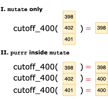
Note that the use of map allows a vector to be returned by the cutoff_400 function, which can then be used as a column in the mutate call.
Pop quiz: In our two examples of applying a function to wt and disp, the new tibble (stored in mtcars_transformed) lost information about the values of wt and disp before the transformation. How could we amend our examples to still preserve the original information in case we would like to make comparisons between the before and after?
2.6 Handling Missing Values
In the section on joining tables together we saw a special value called NA crop up when rows did not align during the matching. We call these special quantities, as you might expect, missing values since they are “holes” in the data. In this section we dive more into missing values and how to address them in your datasets.
2.6.2 A dataset with missing values
The tibble trouble_temps contains temperatures from four cities across three consecutive weeks in the summer.
trouble_temps <- tibble(city = c("Miami", "Boston",
                                 "Seattle", "Arlington"),
                        week1 = c(89, 88, 87, NA),
                        week2 = c(91, NA, 86, 75),
                        week3 = c(88, 85, 88, NA))
trouble_temps
## # A tibble: 4 × 4
## city week1 week2 week3
## <chr> <dbl> <dbl> <dbl>
## 1 Miami 89 91 88
## 2 Boston 88 NA 85
## 3 Seattle 87 86 88
## 4 Arlington NA 75 NAAs you might expect, this tibble contains missing values. We can see that Boston is missing a value from week2 and Arlington is missing values from both week1 and week3, possibly due to some faulty equipment.
2.6.3 Eliminating rows with missing values
If you need to get rid of all rows with NA, you can use drop_na which is part of dplyr.
temps_clean <- trouble_temps |>
  drop_na()
temps_clean
## # A tibble: 2 × 4
## city week1 week2 week3
## <chr> <dbl> <dbl> <dbl>
## 1 Miami 89 91 88
## 2 Seattle 87 86 882.6.4 Filling values by looking at neighbors
There is a way to fill missing values by dragging the non-NA value immediately below an NA to its position. In this manner, all NA’s after the first non-NA will acquire a value. This works when the bottom row does not have an NA.
Let us fill the values using this setting.
trouble_temps |>
  fill(week1:week3, .direction = "up")
## # A tibble: 4 × 4
## city week1 week2 week3
## <chr> <dbl> <dbl> <dbl>
## 1 Miami 89 91 88
## 2 Boston 88 86 85
## 3 Seattle 87 86 88
## 4 Arlington NA 75 NANote how the temperatures for Arlington remain unfilled.
In the case where the bottom row has an NA and the top row does not have an NA, you can drag the values upwards instead.
We can also combine the two actions in a bidirectional manner, either going down and then up or going up and then down.
trouble_temps |>
  fill(week1:week3, .direction = "updown")
## # A tibble: 4 × 4
## city week1 week2 week3
## <chr> <dbl> <dbl> <dbl>
## 1 Miami 89 91 88
## 2 Boston 88 86 85
## 3 Seattle 87 86 88
## 4 Arlington 87 75 88The directional specifications are: “up”, “down”, “updown”, and “downup”. The default direction is “down”, and so you do not have state it.
2.6.5 Filling values according to a global constant
If you want to make an across-the-board replacement of NA with a specific value, you can use the function replace_na from tidyr. For instance, the following replaces missing values in week1 with the value 70.
trouble_temps |>
  mutate(week1 = replace_na(week1, 70))
## # A tibble: 4 × 4
## city week1 week2 week3
## <chr> <dbl> <dbl> <dbl>
## 1 Miami 89 91 88
## 2 Boston 88 NA 85
## 3 Seattle 87 86 88
## 4 Arlington 70 75 NAIf you wish to apply this for all columns in the dataset, we can use provide replace_na as an anonymous function in a combination of mutate with across.
trouble_temps |>
  mutate(across(week1:week3, function(x) replace_na(x, 70)))
## # A tibble: 4 × 4
## city week1 week2 week3
## <chr> <dbl> <dbl> <dbl>
## 1 Miami 89 91 88
## 2 Boston 88 70 85
## 3 Seattle 87 86 88
## 4 Arlington 70 75 70Note that if your dataset contains a mixture of strings and numbers, then a straightforward application like this will not work. Instead, you will need to split the process into two steps: first handling missing values in the strings columns and then, afterwards, taking care of the missing values in the numeric columns.
Alternatively, you can use replace_na to give an instruction how to handle NA appearing in specific columns.
The syntax for the instruction is simple. For each attribute you make a placement, state its name, add an equal sign, and then add the value you want to use for replacement. The replacement instructions must appear in a list, even if there is only one replacement instruction.
Below, we fill any NA in week1 with 89, in week2 with 91, and in week3 with 88.
trouble_temps |>
  replace_na(list(week1 = 89, week2 = 91, week3 = 88))
## # A tibble: 4 × 4
## city week1 week2 week3
## <chr> <dbl> <dbl> <dbl>
## 1 Miami 89 91 88
## 2 Boston 88 91 85
## 3 Seattle 87 86 88
## 4 Arlington 89 75 88Case Study: Tidy Assessments
In this section, we present a larger dataset and apply transformations that are necessary to bring it into tidy data to facilitate further analysis. The goal of this exercise is to demonstrate how the transformations we have learned in this chapter are not tools meant to be used in isolation, but work best when used together to fulfill a complex goal.
Prerequisites
As always, we will need the tidyverse to accomplish our task. We will also load in the edsdata package that contains the datasets we will be working with.
The tibbles csc_course_lab, csc_course_hw, and csc_course_qz
We will examine three datasets that contain assessment results from a hypothetical introductory course in Computer Science. These datasets come from the edsdata package.
csc_course_lab## # A tibble: 116 × 13
## number lab01 lab02 lab03 lab04 lab05 lab06 lab07 lab08 lab09 lab10 lab11
## <dbl> <dbl> <dbl> <dbl> <dbl> <dbl> <dbl> <dbl> <dbl> <dbl> <dbl> <dbl>
## 1 1 10 10 10 10 10 10 10 10 10 10 10
## 2 2 10 10 10 10 10 10 10 10 10 10 10
## 3 3 10 10 10 10 10 10 10 10 10 10 10
## 4 4 10 10 10 10 10 10 10 10 10 10 10
## 5 5 10 10 10 10 10 10 10 10 10 10 10
## 6 6 10 10 10 10 10 10 NA NA 10 10 NA
## 7 7 10 10 10 10 10 10 10 10 10 10 10
## 8 8 10 10 10 10 10 10 10 NA NA 10 10
## 9 9 10 10 10 8 10 10 10 10 10 NA 10
## 10 10 10 10 0 10 10 10 10 NA NA 10 NA
## # ℹ 106 more rows
## # ℹ 1 more variable: lab12 <dbl>
csc_course_hw## # A tibble: 116 × 12
## number hw01 hw02 hw03 hw04 hw05 hw06 hw07 hw08 hw09 hw10 hw11
## <dbl> <dbl> <dbl> <dbl> <dbl> <dbl> <dbl> <dbl> <dbl> <dbl> <dbl> <dbl>
## 1 1 10 10 10 9 10 10 9 10 7 NA 3
## 2 2 10 10 9 10 9 10 6 10 7 10 10
## 3 3 10 8 10 10 9 10 10 10 10 10 NA
## 4 4 10 10 10 10 10 10 9 10 9 10 8
## 5 5 10 10 10 10 10 10 9 10 10 10 7
## 6 6 5 0 9 0 10 NA 8 NA 5 NA NA
## 7 7 10 10 9 10 9 10 8 10 10 10 8
## 8 8 10 10 0 0 NA 10 NA NA NA NA NA
## 9 9 10 9 9 9 10 10 9 10 9 NA NA
## 10 10 8 9 0 0 10 NA NA NA 9 10 NA
## # ℹ 106 more rows
csc_course_qz## # A tibble: 116 × 4
## number qz01 qz02 qz03
## <dbl> <dbl> <dbl> <dbl>
## 1 1 85 100 60
## 2 2 100 90 100
## 3 3 83 92.5 100
## 4 4 100 100 100
## 5 5 97 100 96.7
## 6 6 33 77.5 73.3
## 7 7 90 77.5 100
## 8 8 50.8 47.5 6.67
## 9 9 100 80 80
## 10 10 41 22.5 0
## # ℹ 106 more rowsFollowing is some information about the dataset:
- The
numbercolumn gives a unique number of each student enrolled in the course. - There are ten
labXXattributes (for labs), elevenhwXXattributes (for homeworks), and threeqzXXscores (for quizzes). - The dataset is split across three different tables: one for lab scores, a second for homework scores, and a third for quiz scores.
- The data abounds with missing values. The missing values in this dataset have a clear explanation: some students did not turn in all of the labs and/or assignments.
Let us state the observational unit to be an individual student assessment and we would like to measure the following variables:
- number, a unique number of each student
- assessment, the kind of assessment, e.g., lab01, hw01, qz01
- score, the received score on the assessment
We can see the current format of the dataset violates all three principles of tidy data. Those problems being:
- The observational unit is the student which is spread across three different tables.
- There is missing data present which, by definition, is not tidy.
- We would like to keep the scale of the scores the same for each assessment, i.e., labs, homeworks, and quizzes should all be on a 100 point scale.
- Both the student number and score appears in each column and multiple observations appear in each row.
Once we have tided the data, we would like to answer the following questions:
- What is average lab, homework, and quiz score for each of the students? What are the overall averages for the class?
- Which students performed poorly in the course?
We will address each of these in turn.
Joining like data together
To resolve the first problem, we should merge the data from each of the three tibbles into one single tibble. We know how to do this using the join operation.
We are quite fortunate because each table shares a common attribute which we can use as a key in the join: number. We will coordinate the join by first merging the homework and lab tibbles together, and then merging the resulting tibble with the quiz tibble.
csc_course_merged <- csc_course_hw |>
  inner_join(csc_course_lab, by = "number") |>
  inner_join(csc_course_qz, by = "number")
csc_course_merged
## # A tibble: 116 × 27
## number hw01 hw02 hw03 hw04 hw05 hw06 hw07 hw08 hw09 hw10 hw11
## <dbl> <dbl> <dbl> <dbl> <dbl> <dbl> <dbl> <dbl> <dbl> <dbl> <dbl> <dbl>
## 1 1 10 10 10 9 10 10 9 10 7 NA 3
## 2 2 10 10 9 10 9 10 6 10 7 10 10
## 3 3 10 8 10 10 9 10 10 10 10 10 NA
## 4 4 10 10 10 10 10 10 9 10 9 10 8
## 5 5 10 10 10 10 10 10 9 10 10 10 7
## 6 6 5 0 9 0 10 NA 8 NA 5 NA NA
## 7 7 10 10 9 10 9 10 8 10 10 10 8
## 8 8 10 10 0 0 NA 10 NA NA NA NA NA
## 9 9 10 9 9 9 10 10 9 10 9 NA NA
## 10 10 8 9 0 0 10 NA NA NA 9 10 NA
## # ℹ 106 more rows
## # ℹ 15 more variables: lab01 <dbl>, lab02 <dbl>, lab03 <dbl>, lab04 <dbl>,
## # lab05 <dbl>, lab06 <dbl>, lab07 <dbl>, lab08 <dbl>, lab09 <dbl>,
## # lab10 <dbl>, lab11 <dbl>, lab12 <dbl>, qz01 <dbl>, qz02 <dbl>, qz03 <dbl>Note that even though we used inner_join here, the resulting tibble would have been the same if we had used any of the other styles of join. Why might that be?
Addressing missing data
Now that we have the data in a single table, we can address the problem of missing data. As we noted earlier, the missing values have a meaning in the dataset: the student did not turn in the associated assessment. The appropriate way to handle this is to substitute each missing value with a 0 – sorry folks!
We can accomplish this using the replace_na function. We express the anonymous function that uses replace_na with formula notation.
csc_course_merged <- csc_course_merged |>
  mutate(across(everything(), \(x) replace_na(x, 0)))
csc_course_merged
## # A tibble: 116 × 27
## number hw01 hw02 hw03 hw04 hw05 hw06 hw07 hw08 hw09 hw10 hw11
## <dbl> <dbl> <dbl> <dbl> <dbl> <dbl> <dbl> <dbl> <dbl> <dbl> <dbl> <dbl>
## 1 1 10 10 10 9 10 10 9 10 7 0 3
## 2 2 10 10 9 10 9 10 6 10 7 10 10
## 3 3 10 8 10 10 9 10 10 10 10 10 0
## 4 4 10 10 10 10 10 10 9 10 9 10 8
## 5 5 10 10 10 10 10 10 9 10 10 10 7
## 6 6 5 0 9 0 10 0 8 0 5 0 0
## 7 7 10 10 9 10 9 10 8 10 10 10 8
## 8 8 10 10 0 0 0 10 0 0 0 0 0
## 9 9 10 9 9 9 10 10 9 10 9 0 0
## 10 10 8 9 0 0 10 0 0 0 9 10 0
## # ℹ 106 more rows
## # ℹ 15 more variables: lab01 <dbl>, lab02 <dbl>, lab03 <dbl>, lab04 <dbl>,
## # lab05 <dbl>, lab06 <dbl>, lab07 <dbl>, lab08 <dbl>, lab09 <dbl>,
## # lab10 <dbl>, lab11 <dbl>, lab12 <dbl>, qz01 <dbl>, qz02 <dbl>, qz03 <dbl>Missing values, begone!
Scaling scores to the same point scale
Next, we turn to scaling the points so that everything is on the 100 point scale. To accomplish this, we need to convert all of the labs and homeworks column from a 10 point to a 100 point scale.
To do this, we will apply a function to each of the labs and homeworks columns. Here is the function we will apply.
convert_to_100_points <- function(x) {
  return((x / 10) * 100)
}
We could apply a mutate for each of the eleven homeworks and twelve labs, but this can be quite cumbersome to type. The function across allows us to mutate multiple columns at once. Here is how we can put everything together.
csc_course_merged <- csc_course_merged |>
  mutate(across(matches("lab"), convert_to_100_points),
         across(matches("hw"), convert_to_100_points))
csc_course_merged
## # A tibble: 116 × 27
## number hw01 hw02 hw03 hw04 hw05 hw06 hw07 hw08 hw09 hw10 hw11
## <dbl> <dbl> <dbl> <dbl> <dbl> <dbl> <dbl> <dbl> <dbl> <dbl> <dbl> <dbl>
## 1 1 100 100 100 90 100 100 90 100 70 0 30
## 2 2 100 100 90 100 90 100 60 100 70 100 100
## 3 3 100 80 100 100 90 100 100 100 100 100 0
## 4 4 100 100 100 100 100 100 90 100 90 100 80
## 5 5 100 100 100 100 100 100 90 100 100 100 70
## 6 6 50 0 90 0 100 0 80 0 50 0 0
## 7 7 100 100 90 100 90 100 80 100 100 100 80
## 8 8 100 100 0 0 0 100 0 0 0 0 0
## 9 9 100 90 90 90 100 100 90 100 90 0 0
## 10 10 80 90 0 0 100 0 0 0 90 100 0
## # ℹ 106 more rows
## # ℹ 15 more variables: lab01 <dbl>, lab02 <dbl>, lab03 <dbl>, lab04 <dbl>,
## # lab05 <dbl>, lab06 <dbl>, lab07 <dbl>, lab08 <dbl>, lab09 <dbl>,
## # lab10 <dbl>, lab11 <dbl>, lab12 <dbl>, qz01 <dbl>, qz02 <dbl>, qz03 <dbl>Note that the function matches("lab") looks for all columns that have the name "lab" in it, which will return the twelve lab columns. Ditto matches("hw") and the homework columns.
Pivoting
We will now resolve our fourth stated problem. To overcome this, we can use the pivot transformation so that the three variables become apparent in the table: number, assessment, and score.
csc_course_merged <- csc_course_merged |>
  pivot_longer(starts_with("hw") |
                 starts_with("lab") | starts_with("qz"),
               names_to = "assessment", values_to = "score")
csc_course_merged
## # A tibble: 3,016 × 3
## number assessment score
## <dbl> <chr> <dbl>
## 1 1 hw01 100
## 2 1 hw02 100
## 3 1 hw03 100
## 4 1 hw04 90
## 5 1 hw05 100
## 6 1 hw06 100
## 7 1 hw07 90
## 8 1 hw08 100
## 9 1 hw09 70
## 10 1 hw10 0
## # ℹ 3,006 more rowsThe one bit of machinery we added here is the Boolean expression starts_with("hw") | starts_with("lab") | starts_with("qz") so that we are able to select all of the homework, lab, and quiz columns at once. The meaning of this expression should be straightforward.
This data is just about tidied. The difference between the individual assessments, e.g., “hw01” versus “hw03”, does not concern us for this analysis, so let us tidy the values in the assessment column so that only three values appear: hw, lab, and qz.
We can use a regular expression in a call to str_replace to do the work for us. Here is an example of the regular expression in action.
str_view_all("hw05", "[0-9]+")## Warning: `str_view_all()` was deprecated in stringr 1.5.0.
## ℹ Please use `str_view()` instead.
## This warning is displayed once every 8 hours.
## Call `lifecycle::last_lifecycle_warnings()` to see where this warning was
## generated.## [1] │ hw<05>Once we have matched any of the numerical characters, we can replace them with an empty string "". For instance:
str_replace("hw05", "[0-9]+", "")## [1] "hw"We can now pull everything together using a call to mutate.
csc_course_merged <- csc_course_merged |>
  mutate(assessment = str_replace(assessment, "[0-9]+", ""))
csc_course_merged
## # A tibble: 3,016 × 3
## number assessment score
## <dbl> <chr> <dbl>
## 1 1 hw 100
## 2 1 hw 100
## 3 1 hw 100
## 4 1 hw 90
## 5 1 hw 100
## 6 1 hw 100
## 7 1 hw 90
## 8 1 hw 100
## 9 1 hw 70
## 10 1 hw 0
## # ℹ 3,006 more rowsLooks great! Let us finish by answering some questions about the data.
The good stuff: summarizing information
We are now ready to answer some of the questions we proposed at the outset of this section. Our first question: what is average lab, homework, and quiz score for each of the students; what are the overall averages for the class?
We can answer this using a combination of the group_by and summarize verbs. We will group by the variables number and assessment and then summarize the grouped means for each group.
## # A tibble: 348 × 3
## # Groups:   number [116]
##    number assessment mean_score
##     <dbl> <chr>           <dbl>
##  1      1 hw               80
##  2      1 lab              91.7
##  3      1 qz               81.7
##  4      2 hw               91.8
##  5      2 lab             100
##  6      2 qz               96.7
##  7      3 hw               88.2
##  8      3 lab              91.7
##  9      3 qz               91.8
## 10      4 hw               96.4
## # ℹ 338 more rows
Compare this table with the previous and note how there is only one hw, lab, and qz assessment for each student. The reported value that you see is the mean score for all of the assessments in that category for the student, e.g., the first row shows their average homework score over the eleven homeworks.
Let us go further and report the overall assessment averages.
## # A tibble: 3 × 2
##   assessment mean_score
##   <chr>           <dbl>
## 1 hw               78.2
## 2 lab              91.4
## 3 qz               78.4
Neat! Users of Excel or spreadsheet software might find a result like this familiar.
Assuming that each assessment is weighted equally, let us find the mean score for each of the students.
csc_summary <- csc_course_merged |>
  group_by(number) |>
  summarize(mean_overall_score = mean(score))
csc_summary
## # A tibble: 116 × 2
## number mean_overall_score
## <dbl> <dbl>
## 1 1 85.6
## 2 2 96.2
## 3 3 90.2
## 4 4 98.5
## 5 5 98.2
## 6 6 52.1
## 7 7 96.4
## 8 8 54.0
## 9 9 84.2
## 10 10 47.1
## # ℹ 106 more rowsNow let us zoom in on those that are performing less than, say, 70.
csc_summary |>
  filter(mean_overall_score < 70)
## # A tibble: 16 × 2
## number mean_overall_score
## <dbl> <dbl>
## 1 6 52.1
## 2 8 54.0
## 3 10 47.1
## 4 17 52.1
## 5 18 61.7
## 6 20 68.1
## 7 31 15.4
## 8 32 10.4
## 9 38 68.9
## 10 41 68.1
## 11 45 67.3
## 12 61 60
## 13 98 56.9
## 14 104 55.2
## 15 107 36.9
## 16 112 51.1You can imagine how such an analysis could be useful when used mid-semester – we could check in with those students to investigate further.
Case Study: Exploring the College Scorecard
Before closing the chapter, we present one more application of data transformation techniques in a real-world setting. This time, we turn to a much larger dataset and appeal to the annual College Scorecard published by the Department of Education on recent institution-level data. We will use this dataset to explore the average annual cost of attending public and private institutions in the Miami area.
Prerequisites
As before, let us load tidyverse.
The full data is available for download here, however, we have already done some basic preprocessing of this dataset by including only Florida-based institutions. This tibble is available in scorecard_fl from the edsdata package. Let us have a look at the data:
scorecard_fl## # A tibble: 395 × 2,989
## UNITID OPEID OPEID6 INSTNM CITY STABBR ZIP ACCREDAGENCY INSTURL NPCURL
## <int> <chr> <chr> <chr> <chr> <chr> <chr> <chr> <chr> <chr>
## 1 132374 01226300 012263 Atlant… Coco… FL 3306… Council on … www.at… www.a…
## 2 132408 02159600 021596 The Ba… Grac… FL 32440 Southern As… www.ba… www.b…
## 3 132471 00146600 001466 Barry … Miami FL 3316… Southern As… www.ba… www.b…
## 4 132602 00146700 001467 Bethun… Dayt… FL 3211… Southern As… www.co… nces.…
## 5 132657 00150500 001505 Lynn U… Boca… FL 3343… Southern As… www.ly… https…
## 6 132675 03382300 033823 North … Star… FL 32091 Council on … www.nf… nftc.…
## 7 132693 00147000 001470 Easter… Cocoa FL 32922 Southern As… www.ea… www.e…
## 8 132709 00150000 001500 Browar… Fort… FL 33301 Southern As… www.br… www.b…
## 9 132842 01072401 010724 Albizu… Miami FL 3317… Middle Stat… https:… https…
## 10 132851 00147100 001471 Colleg… Ocala FL 34474 Southern As… www.cf… https…
## # ℹ 385 more rows
## # ℹ 2,979 more variables: SCH_DEG <chr>, HCM2 <int>, MAIN <int>,
## # NUMBRANCH <int>, PREDDEG <int>, HIGHDEG <int>, CONTROL <int>,
## # ST_FIPS <int>, REGION <int>, LOCALE <chr>, LOCALE2 <chr>, LATITUDE <chr>,
## # LONGITUDE <chr>, CCBASIC <chr>, CCUGPROF <chr>, CCSIZSET <chr>, HBCU <chr>,
## # PBI <chr>, ANNHI <chr>, TRIBAL <chr>, AANAPII <chr>, HSI <chr>,
## # NANTI <chr>, MENONLY <chr>, WOMENONLY <chr>, RELAFFIL <chr>, …The information is divided into small specific categories. Have a look at the accompanying glossary and data dictionary to learn more about the variables in the dataset. You can also download it to learn about what each variable represents and the corresponding data types.
Indeed, the number of variables present in this dataset is very large (2,989) and certainly beyond any inspection we could accomplish by hand.
Net Tuition of Four-Year Institutions in Miami
We will concentrate specifically on variables that correspond to the average net price for students who receive some kind of financial aid for one year of academic study. Therefore, we will collect the following from the large number of variables present in the dataset:
- Institution name (
INSTNM) - City of location (
CITY) - State of location (
STABBR) - Zipcode (
ZIP) - Number of undergraduate students (
UGDS) - Four-year net tuition in the case of a public institution (
NPT4_PUB) - Four-year net tuition in the case of a private institution (
NPT4_PRIV)
Note that the last two variables have different names, but they both represent the net tuition. We drill down the tibble to contain just these variables:
scorecard_relevant <- scorecard_fl |>
  select(INSTNM:NPT4_PRIV)
scorecard_relevant
## # A tibble: 395 × 315
## INSTNM CITY STABBR ZIP ACCREDAGENCY INSTURL NPCURL SCH_DEG HCM2 MAIN
## <chr> <chr> <chr> <chr> <chr> <chr> <chr> <chr> <int> <int>
## 1 Atlantic … Coco… FL 3306… Council on … www.at… www.a… 1 0 1
## 2 The Bapti… Grac… FL 32440 Southern As… www.ba… www.b… 3 0 1
## 3 Barry Uni… Miami FL 3316… Southern As… www.ba… www.b… 3 0 1
## 4 Bethune-C… Dayt… FL 3211… Southern As… www.co… nces.… 3 0 1
## 5 Lynn Univ… Boca… FL 3343… Southern As… www.ly… https… 3 0 1
## 6 North Flo… Star… FL 32091 Council on … www.nf… nftc.… 1 0 1
## 7 Eastern F… Cocoa FL 32922 Southern As… www.ea… www.e… 2 0 1
## 8 Broward C… Fort… FL 33301 Southern As… www.br… www.b… 2 0 1
## 9 Albizu Un… Miami FL 3317… Middle Stat… https:… https… 3 0 0
## 10 College o… Ocala FL 34474 Southern As… www.cf… https… 2 0 1
## # ℹ 385 more rows
## # ℹ 305 more variables: NUMBRANCH <int>, PREDDEG <int>, HIGHDEG <int>,
## # CONTROL <int>, ST_FIPS <int>, REGION <int>, LOCALE <chr>, LOCALE2 <chr>,
## # LATITUDE <chr>, LONGITUDE <chr>, CCBASIC <chr>, CCUGPROF <chr>,
## # CCSIZSET <chr>, HBCU <chr>, PBI <chr>, ANNHI <chr>, TRIBAL <chr>,
## # AANAPII <chr>, HSI <chr>, NANTI <chr>, MENONLY <chr>, WOMENONLY <chr>,
## # RELAFFIL <chr>, ADM_RATE <chr>, ADM_RATE_ALL <chr>, SATVR25 <chr>, …For the purposes of this analysis, we would like to perform the following to bring this data into tidy format:
- Form a single representation of the net tuition where the distinction between a “public” tuition and a “private” tuition does not matter. At the moment, this variable is split across two columns.
- Standardize the ZIP codes so that it contains only the first five digit specification and not the ZIP+4 specification.
- Filter down the institutions to those that are based in Miami.
- Create a dedicated column that expresses whether the institution is private or public.
Handling missing values
We would like to focus only on those institutions that have a recorded four-year net tuition (public or private). We would expect, then, to be able to eliminate the observations that do not by keeping only those observations where a missing value is not present in one of the two net tuition variables (NPT4_PUB and NPT4_PRIV).
## # A tibble: 395 × 315
##    INSTNM     CITY  STABBR ZIP   ACCREDAGENCY INSTURL NPCURL SCH_DEG  HCM2  MAIN
##    <chr>      <chr> <chr>  <chr> <chr>        <chr>   <chr>  <chr>   <int> <int>
##  1 Atlantic … Coco… FL     3306… Council on … www.at… www.a… 1           0     1
##  2 The Bapti… Grac… FL     32440 Southern As… www.ba… www.b… 3           0     1
##  3 Barry Uni… Miami FL     3316… Southern As… www.ba… www.b… 3           0     1
##  4 Bethune-C… Dayt… FL     3211… Southern As… www.co… nces.… 3           0     1
##  5 Lynn Univ… Boca… FL     3343… Southern As… www.ly… https… 3           0     1
##  6 North Flo… Star… FL     32091 Council on … www.nf… nftc.… 1           0     1
##  7 Eastern F… Cocoa FL     32922 Southern As… www.ea… www.e… 2           0     1
##  8 Broward C… Fort… FL     33301 Southern As… www.br… www.b… 2           0     1
##  9 Albizu Un… Miami FL     3317… Middle Stat… https:… https… 3           0     0
## 10 College o… Ocala FL     34474 Southern As… www.cf… https… 2           0     1
## # ℹ 385 more rows
## # ℹ 305 more variables: NUMBRANCH <int>, PREDDEG <int>, HIGHDEG <int>,
## #   CONTROL <int>, ST_FIPS <int>, REGION <int>, LOCALE <chr>, LOCALE2 <chr>,
## #   LATITUDE <chr>, LONGITUDE <chr>, CCBASIC <chr>, CCUGPROF <chr>,
## #   CCSIZSET <chr>, HBCU <chr>, PBI <chr>, ANNHI <chr>, TRIBAL <chr>,
## #   AANAPII <chr>, HSI <chr>, NANTI <chr>, MENONLY <chr>, WOMENONLY <chr>,
## # RELAFFIL <chr>, ADM_RATE <chr>, ADM_RATE_ALL <chr>, SATVR25 <chr>, …It would seem all is well and that the data we have is indeed complete. However, a closer look at one of the institutions tells all:
scorecard_relevant |>
  filter(INSTNM == "Florida Institute of Ultrasound Inc")
## # A tibble: 1 × 315
## INSTNM NPT4_PUB NPT4_PRIV CITY STABBR ZIP ACCREDAGENCY INSTURL NPCURL
## <chr> <chr> <chr> <chr> <chr> <chr> <chr> <chr> <chr>
## 1 Florida Ins… NULL NULL Pens… FL 32514 NULL www.fi… www.f…
## # ℹ 306 more variables: SCH_DEG <chr>, HCM2 <int>, MAIN <int>, NUMBRANCH <int>,
## # PREDDEG <int>, HIGHDEG <int>, CONTROL <int>, ST_FIPS <int>, REGION <int>,
## # LOCALE <chr>, LOCALE2 <chr>, LATITUDE <chr>, LONGITUDE <chr>,
## # CCBASIC <chr>, CCUGPROF <chr>, CCSIZSET <chr>, HBCU <chr>, PBI <chr>,
## # ANNHI <chr>, TRIBAL <chr>, AANAPII <chr>, HSI <chr>, NANTI <chr>,
## # MENONLY <chr>, WOMENONLY <chr>, RELAFFIL <chr>, ADM_RATE <chr>,
## # ADM_RATE_ALL <chr>, SATVR25 <chr>, SATVR75 <chr>, SATMT25 <chr>, …The College Scorecard chooses to present missing values in a non-standard form using the special string "NULL". While human users of this table will have no trouble understanding the meaning of this keyword, R is unable to distinguish "NULL" from any other string that may be present. Therefore, as far as our dplyr code is concerned, there are no “missing values” in this dataset.
We can remedy the problem by converting all instances of "NULL" that may appear in a string column to proper missing values so that these can be detected appropriately by our dplyr verbs. The function we use is na_if, which is similar to the replace_na function shown earlier. Note that this transformation is applied specifically to all string columns using the helper dplyr verb where.
scorecard_relevant <- scorecard_relevant |>
  mutate(across(where(is_character), \(x) na_if(x, "NULL")))
By running our prior code chunk again, the irrelevant institutions are now properly removed.
## # A tibble: 290 × 315
##    INSTNM     CITY  STABBR ZIP   ACCREDAGENCY INSTURL NPCURL SCH_DEG  HCM2  MAIN
##    <chr>      <chr> <chr>  <chr> <chr>        <chr>   <chr>  <chr>   <int> <int>
##  1 Atlantic … Coco… FL     3306… Council on … www.at… www.a… 1           0     1
##  2 The Bapti… Grac… FL     32440 Southern As… www.ba… www.b… 3           0     1
##  3 Barry Uni… Miami FL     3316… Southern As… www.ba… www.b… 3           0     1
##  4 Bethune-C… Dayt… FL     3211… Southern As… www.co… nces.… 3           0     1
##  5 Lynn Univ… Boca… FL     3343… Southern As… www.ly… https… 3           0     1
##  6 North Flo… Star… FL     32091 Council on … www.nf… nftc.… 1           0     1
##  7 Eastern F… Cocoa FL     32922 Southern As… www.ea… www.e… 2           0     1
##  8 Broward C… Fort… FL     33301 Southern As… www.br… www.b… 2           0     1
##  9 Albizu Un… Miami FL     3317… Middle Stat… https:… https… 3           0     0
## 10 College o… Ocala FL     34474 Southern As… www.cf… https… 2           0     1
## # ℹ 280 more rows
## # ℹ 305 more variables: NUMBRANCH <int>, PREDDEG <int>, HIGHDEG <int>,
## #   CONTROL <int>, ST_FIPS <int>, REGION <int>, LOCALE <chr>, LOCALE2 <chr>,
## #   LATITUDE <chr>, LONGITUDE <chr>, CCBASIC <chr>, CCUGPROF <chr>,
## #   CCSIZSET <chr>, HBCU <chr>, PBI <chr>, ANNHI <chr>, TRIBAL <chr>,
## #   AANAPII <chr>, HSI <chr>, NANTI <chr>, MENONLY <chr>, WOMENONLY <chr>,
## #   RELAFFIL <chr>, ADM_RATE <chr>, ADM_RATE_ALL <chr>, SATVR25 <chr>, …
We can combine our steps to form a strategy for handling missing values in this dataset. While we are at it, we will convert the net tuition columns to double columns as these express numerical quantities and not strings.
with_net_tuition <- scorecard_relevant |>
  mutate(across(where(is_character), \(x) na_if(x, "NULL"))) |>
  filter(!is.na(NPT4_PUB) | !is.na(NPT4_PRIV)) |>
  mutate(NPT4_PUB = as.double(NPT4_PUB),
         NPT4_PRIV = as.double(NPT4_PRIV))
with_net_tuition
## # A tibble: 290 × 315
## INSTNM CITY STABBR ZIP ACCREDAGENCY INSTURL NPCURL SCH_DEG HCM2 MAIN
## <chr> <chr> <chr> <chr> <chr> <chr> <chr> <chr> <int> <int>
## 1 Atlantic … Coco… FL 3306… Council on … www.at… www.a… 1 0 1
## 2 The Bapti… Grac… FL 32440 Southern As… www.ba… www.b… 3 0 1
## 3 Barry Uni… Miami FL 3316… Southern As… www.ba… www.b… 3 0 1
## 4 Bethune-C… Dayt… FL 3211… Southern As… www.co… nces.… 3 0 1
## 5 Lynn Univ… Boca… FL 3343… Southern As… www.ly… https… 3 0 1
## 6 North Flo… Star… FL 32091 Council on … www.nf… nftc.… 1 0 1
## 7 Eastern F… Cocoa FL 32922 Southern As… www.ea… www.e… 2 0 1
## 8 Broward C… Fort… FL 33301 Southern As… www.br… www.b… 2 0 1
## 9 Albizu Un… Miami FL 3317… Middle Stat… https:… https… 3 0 0
## 10 College o… Ocala FL 34474 Southern As… www.cf… https… 2 0 1
## # ℹ 280 more rows
## # ℹ 305 more variables: NUMBRANCH <int>, PREDDEG <int>, HIGHDEG <int>,
## # CONTROL <int>, ST_FIPS <int>, REGION <int>, LOCALE <chr>, LOCALE2 <chr>,
## # LATITUDE <chr>, LONGITUDE <chr>, CCBASIC <chr>, CCUGPROF <chr>,
## # CCSIZSET <chr>, HBCU <chr>, PBI <chr>, ANNHI <chr>, TRIBAL <chr>,
## # AANAPII <chr>, HSI <chr>, NANTI <chr>, MENONLY <chr>, WOMENONLY <chr>,
## # RELAFFIL <chr>, ADM_RATE <chr>, ADM_RATE_ALL <chr>, SATVR25 <chr>, …ZIP code information
We turn to cleaning the ZIP code information in the dataset. Let us examine some of these ZIP codes in ZIP:
with_net_tuition |>
  select(ZIP)
## # A tibble: 290 × 1
## ZIP
## <chr>
## 1 33063-3902
## 2 32440
## 3 33161-6695
## 4 32114-3099
## 5 33431-5598
## 6 32091
## 7 32922
## 8 33301
## 9 33172-2209
## 10 34474
## # ℹ 280 more rowsAs the table snippet shows, some of the ZIP codes are given using the 5 digit specification (e.g., 32440) and others using the ZIP+4 specification (e.g., 33063-3902).
We can standardize the ZIP codes using functionality from stringr. The following extracts just the 5 digit specification from representations that may be present:
str_replace(c("33172-2209", "34474"), "\\-[:number:]+", "")## [1] "33172" "34474"We replace the column ZIP with the cleaned zip code format.
with_net_tuition |>
  mutate(ZIP5 = str_replace(ZIP, "\\-[:number:]+", "")) |>
  relocate(ZIP5, .before = CITY)
## # A tibble: 290 × 316
## INSTNM ZIP5 CITY STABBR ZIP ACCREDAGENCY INSTURL NPCURL SCH_DEG HCM2
## <chr> <chr> <chr> <chr> <chr> <chr> <chr> <chr> <chr> <int>
## 1 Atlantic … 33063 Coco… FL 3306… Council on … www.at… www.a… 1 0
## 2 The Bapti… 32440 Grac… FL 32440 Southern As… www.ba… www.b… 3 0
## 3 Barry Uni… 33161 Miami FL 3316… Southern As… www.ba… www.b… 3 0
## 4 Bethune-C… 32114 Dayt… FL 3211… Southern As… www.co… nces.… 3 0
## 5 Lynn Univ… 33431 Boca… FL 3343… Southern As… www.ly… https… 3 0
## 6 North Flo… 32091 Star… FL 32091 Council on … www.nf… nftc.… 1 0
## 7 Eastern F… 32922 Cocoa FL 32922 Southern As… www.ea… www.e… 2 0
## 8 Broward C… 33301 Fort… FL 33301 Southern As… www.br… www.b… 2 0
## 9 Albizu Un… 33172 Miami FL 3317… Middle Stat… https:… https… 3 0
## 10 College o… 34474 Ocala FL 34474 Southern As… www.cf… https… 2 0
## # ℹ 280 more rows
## # ℹ 306 more variables: MAIN <int>, NUMBRANCH <int>, PREDDEG <int>,
## # HIGHDEG <int>, CONTROL <int>, ST_FIPS <int>, REGION <int>, LOCALE <chr>,
## # LOCALE2 <chr>, LATITUDE <chr>, LONGITUDE <chr>, CCBASIC <chr>,
## # CCUGPROF <chr>, CCSIZSET <chr>, HBCU <chr>, PBI <chr>, ANNHI <chr>,
## # TRIBAL <chr>, AANAPII <chr>, HSI <chr>, NANTI <chr>, MENONLY <chr>,
## # WOMENONLY <chr>, RELAFFIL <chr>, ADM_RATE <chr>, ADM_RATE_ALL <chr>, …We add a step to this sequence where we zoom in on institutions that are Miami-based. We can accomplish this by filtering ZIP codes that begin with "331".
with_clean_zip <- with_net_tuition |>
  mutate(ZIP = str_replace(ZIP, "\\-[:number:]+", "")) |>
  relocate(ZIP, .before = CITY) |>
  filter(str_starts(ZIP, "331"))
with_clean_zip
## # A tibble: 46 × 315
## INSTNM ZIP CITY STABBR ACCREDAGENCY INSTURL NPCURL SCH_DEG HCM2 MAIN
## <chr> <chr> <chr> <chr> <chr> <chr> <chr> <chr> <int> <int>
## 1 Barry Uni… 33161 Miami FL Southern As… www.ba… www.b… 3 0 1
## 2 Albizu Un… 33172 Miami FL Middle Stat… https:… https… 3 0 0
## 3 Florida I… 33199 Miami FL Southern As… www.fi… finan… 3 0 1
## 4 Florida C… 33174 Miami FL Council on … https:… https… 1 0 1
## 5 George T … 33142 Miami FL Council on … https:… https… 1 0 1
## 6 AI Miami … 33132 Miami FL Southern As… www.ar… https… 3 1 1
## 7 Lindsey H… 33127 Miami FL Council on … www.li… www.l… 1 0 1
## 8 Miami Dad… 33132 Miami FL Southern As… www.md… www.m… 2 0 1
## 9 Universit… 33146 Cora… FL Southern As… www.mi… https… 3 0 1
## 10 Robert Mo… 33177 Miami FL Council on … rmec.d… rmec.… 1 0 1
## # ℹ 36 more rows
## # ℹ 305 more variables: NUMBRANCH <int>, PREDDEG <int>, HIGHDEG <int>,
## # CONTROL <int>, ST_FIPS <int>, REGION <int>, LOCALE <chr>, LOCALE2 <chr>,
## # LATITUDE <chr>, LONGITUDE <chr>, CCBASIC <chr>, CCUGPROF <chr>,
## # CCSIZSET <chr>, HBCU <chr>, PBI <chr>, ANNHI <chr>, TRIBAL <chr>,
## # AANAPII <chr>, HSI <chr>, NANTI <chr>, MENONLY <chr>, WOMENONLY <chr>,
## # RELAFFIL <chr>, ADM_RATE <chr>, ADM_RATE_ALL <chr>, SATVR25 <chr>, …Uniting the tuition columns
Next, we unite the net tuition columns together into a single new column named NPT4. We can accomplish this work using the tidyr verb unite.
with_clean_zip |>
  unite("NPT4", NPT4_PUB:NPT4_PRIV, na.rm = TRUE)
## # A tibble: 46 × 314
## INSTNM ZIP CITY STABBR ACCREDAGENCY INSTURL NPCURL SCH_DEG HCM2 MAIN
## <chr> <chr> <chr> <chr> <chr> <chr> <chr> <chr> <int> <int>
## 1 Barry Uni… 33161 Miami FL Southern As… www.ba… www.b… 3 0 1
## 2 Albizu Un… 33172 Miami FL Middle Stat… https:… https… 3 0 0
## 3 Florida I… 33199 Miami FL Southern As… www.fi… finan… 3 0 1
## 4 Florida C… 33174 Miami FL Council on … https:… https… 1 0 1
## 5 George T … 33142 Miami FL Council on … https:… https… 1 0 1
## 6 AI Miami … 33132 Miami FL Southern As… www.ar… https… 3 1 1
## 7 Lindsey H… 33127 Miami FL Council on … www.li… www.l… 1 0 1
## 8 Miami Dad… 33132 Miami FL Southern As… www.md… www.m… 2 0 1
## 9 Universit… 33146 Cora… FL Southern As… www.mi… https… 3 0 1
## 10 Robert Mo… 33177 Miami FL Council on … rmec.d… rmec.… 1 0 1
## # ℹ 36 more rows
## # ℹ 304 more variables: NUMBRANCH <int>, PREDDEG <int>, HIGHDEG <int>,
## # CONTROL <int>, ST_FIPS <int>, REGION <int>, LOCALE <chr>, LOCALE2 <chr>,
## # LATITUDE <chr>, LONGITUDE <chr>, CCBASIC <chr>, CCUGPROF <chr>,
## # CCSIZSET <chr>, HBCU <chr>, PBI <chr>, ANNHI <chr>, TRIBAL <chr>,
## # AANAPII <chr>, HSI <chr>, NANTI <chr>, MENONLY <chr>, WOMENONLY <chr>,
## # RELAFFIL <chr>, ADM_RATE <chr>, ADM_RATE_ALL <chr>, SATVR25 <chr>, …However, before uniting we would like to form a new column named ISPUB that indicates whether a given institution is a public or private entity. Moreover, the tuition amounts are currently expressed as character sequences in R (observe the chr data type associated with this column) when these are actually integer quanities. We should convert the newly created NPT4 to an integer column by using as.integer.
Thus, we have the following steps to bring the tuition amounts into a tidy format:
tuition_tidy <- with_clean_zip |>
  mutate(ISPUB = !(is.na(NPT4_PUB))) |>
  unite("NPT4", NPT4_PUB:NPT4_PRIV, na.rm = TRUE) |>
  mutate(NPT4 = as.integer(NPT4))
tuition_tidy
## # A tibble: 46 × 315
## INSTNM ZIP CITY STABBR ACCREDAGENCY INSTURL NPCURL SCH_DEG HCM2 MAIN
## <chr> <chr> <chr> <chr> <chr> <chr> <chr> <chr> <int> <int>
## 1 Barry Uni… 33161 Miami FL Southern As… www.ba… www.b… 3 0 1
## 2 Albizu Un… 33172 Miami FL Middle Stat… https:… https… 3 0 0
## 3 Florida I… 33199 Miami FL Southern As… www.fi… finan… 3 0 1
## 4 Florida C… 33174 Miami FL Council on … https:… https… 1 0 1
## 5 George T … 33142 Miami FL Council on … https:… https… 1 0 1
## 6 AI Miami … 33132 Miami FL Southern As… www.ar… https… 3 1 1
## 7 Lindsey H… 33127 Miami FL Council on … www.li… www.l… 1 0 1
## 8 Miami Dad… 33132 Miami FL Southern As… www.md… www.m… 2 0 1
## 9 Universit… 33146 Cora… FL Southern As… www.mi… https… 3 0 1
## 10 Robert Mo… 33177 Miami FL Council on … rmec.d… rmec.… 1 0 1
## # ℹ 36 more rows
## # ℹ 305 more variables: NUMBRANCH <int>, PREDDEG <int>, HIGHDEG <int>,
## # CONTROL <int>, ST_FIPS <int>, REGION <int>, LOCALE <chr>, LOCALE2 <chr>,
## # LATITUDE <chr>, LONGITUDE <chr>, CCBASIC <chr>, CCUGPROF <chr>,
## # CCSIZSET <chr>, HBCU <chr>, PBI <chr>, ANNHI <chr>, TRIBAL <chr>,
## # AANAPII <chr>, HSI <chr>, NANTI <chr>, MENONLY <chr>, WOMENONLY <chr>,
## # RELAFFIL <chr>, ADM_RATE <chr>, ADM_RATE_ALL <chr>, SATVR25 <chr>, …ZIP code versus net tuition
With our tibble in tidy format, we are ready to use it for data analysis. We are interested in learning more about the following:
- What is the average net tuition for public and private institutions in each zip code area? Which ZIP codes see the highest average net tuition?
- Are private institutions more expensive to attend in the Miami area?
- Which institutions are below the average net tuition for that ZIP code area?
The first two points can be addressed using the following dplyr work. We group observations by ZIP code and type of institution, compute the mean net tuition for each group, and sort the table according to these values.
tuition_tidy |>
  group_by(ZIP, ISPUB) |>
  summarize(NPT4_AVE = mean(NPT4)) |>
  ungroup() |>
  arrange(desc(NPT4_AVE))
## `summarise()` has grouped output by 'ZIP'. You can override using the `.groups`
## argument.## # A tibble: 29 × 3
## ZIP ISPUB NPT4_AVE
## <chr> <lgl> <dbl>
## 1 33146 FALSE 46098
## 2 33165 FALSE 35190
## 3 33176 FALSE 30631
## 4 33126 FALSE 28645
## 5 33174 FALSE 26974.
## 6 33122 FALSE 26389
## 7 33172 FALSE 25210
## 8 33166 FALSE 23792
## 9 33157 FALSE 23343
## 10 33155 FALSE 21988
## # ℹ 19 more rowsIndeed, the top ranking ZIP code areas are dominated by private entities. We can also see that the most expensive area is 33146, where the authors’ home institution resides.
tuition_tidy |>
  filter(ZIP == "33146")
## # A tibble: 1 × 315
## INSTNM ZIP CITY STABBR ACCREDAGENCY INSTURL NPCURL SCH_DEG HCM2 MAIN
## <chr> <chr> <chr> <chr> <chr> <chr> <chr> <chr> <int> <int>
## 1 University… 33146 Cora… FL Southern As… www.mi… https… 3 0 1
## # ℹ 305 more variables: NUMBRANCH <int>, PREDDEG <int>, HIGHDEG <int>,
## # CONTROL <int>, ST_FIPS <int>, REGION <int>, LOCALE <chr>, LOCALE2 <chr>,
## # LATITUDE <chr>, LONGITUDE <chr>, CCBASIC <chr>, CCUGPROF <chr>,
## # CCSIZSET <chr>, HBCU <chr>, PBI <chr>, ANNHI <chr>, TRIBAL <chr>,
## # AANAPII <chr>, HSI <chr>, NANTI <chr>, MENONLY <chr>, WOMENONLY <chr>,
## # RELAFFIL <chr>, ADM_RATE <chr>, ADM_RATE_ALL <chr>, SATVR25 <chr>,
## # SATVR75 <chr>, SATMT25 <chr>, SATMT75 <chr>, SATWR25 <chr>, …For the third point, we can compute the difference of an institution’s net tuition from the mean net tuition in that ZIP code area. We accomplish the work using a grouped mutate.
tuition_tidy |>
  group_by(ZIP) |>
  mutate(NPT4_avg = mean(NPT4),
         tuition_diff = NPT4 - NPT4_avg) |>
  ungroup() |>
  arrange(tuition_diff) |>
  relocate(ISPUB, .before = ZIP)
## # A tibble: 46 × 317
## INSTNM ISPUB ZIP CITY STABBR ACCREDAGENCY INSTURL NPCURL SCH_DEG HCM2
## <chr> <lgl> <chr> <chr> <chr> <chr> <chr> <chr> <chr> <int>
## 1 Prestige … FALSE 33160 Nort… FL Council on … phabsa… phabs… 1 0
## 2 Celebrity… FALSE 33144 Miami FL National Ac… www.ce… celeb… 1 0
## 3 San Ignac… FALSE 33178 Doral FL Accrediting… www.sa… www.s… 2 0
## 4 Miami Dad… TRUE 33132 Miami FL Southern As… www.md… www.m… 2 0
## 5 CBT Techn… FALSE 33157 Cutl… FL Accrediting… www.cb… www.c… 1 0
## 6 CBT Techn… FALSE 33144 Miami FL Accrediting… www.cb… www.c… 1 0
## 7 South Flo… FALSE 33125 Miami FL Accrediting… www.sf… www.s… 1 0
## 8 InterAmer… FALSE 33174 Miami FL Accrediting… www.it… iti.e… 1 0
## 9 New Profe… FALSE 33134 Miami FL Accrediting… www.np… https… 1 0
## 10 Nouvelle … FALSE 33125 Miami FL National Ac… nouvel… nouve… 1 0
## # ℹ 36 more rows
## # ℹ 307 more variables: MAIN <int>, NUMBRANCH <int>, PREDDEG <int>,
## # HIGHDEG <int>, CONTROL <int>, ST_FIPS <int>, REGION <int>, LOCALE <chr>,
## # LOCALE2 <chr>, LATITUDE <chr>, LONGITUDE <chr>, CCBASIC <chr>,
## # CCUGPROF <chr>, CCSIZSET <chr>, HBCU <chr>, PBI <chr>, ANNHI <chr>,
## # TRIBAL <chr>, AANAPII <chr>, HSI <chr>, NANTI <chr>, MENONLY <chr>,
## # WOMENONLY <chr>, RELAFFIL <chr>, ADM_RATE <chr>, ADM_RATE_ALL <chr>, …We can see that a public institution, Miami Dade College, appears toward the top of this ranking.
Because ZIP codes correspond to geographic locations, a possibility for further study would be to overlay the net tuition dataset with spatial information. We could then plot a map of the South Florida and Miami areas and see if the plot reveals any “hot spots”, i.e., areas with unusually high annual costs relative to neighboring ZIP codes. This would add a geographical context for our data points which could suggest new questions for data exploration.
Learning how to plot maps and generate visualizations of tibbles is the subject of the next chapter.
2.7 Exercises
Be sure to install and load the following packages into your R environment before beginning this exercise set.
Question 1 Recall from the textbook that data is tidy when it satisfies four conditions:
2. Each observation forms a row.
3. Each value must have its own cell.
4. Each type of observational unit forms a table.
is_it_tidy <- list(table5, table1, table3, table2)is_it_tidy is a list containing 4 tibbles, with each dataset showing the same values of the four variables country, year, population, and cases, but each dataset organizing the values in a different way. All display the number of Tuberculosis (TB) cases documented by the World Health Organization in Afghanistan, Brazil, and China between 1999 and 2000.
Table 1
is_it_tidy[[1]] # Table 1 Table 2
is_it_tidy[[2]] # Table 2Table 3
is_it_tidy[[3]] # Table 3Table 4
is_it_tidy[[4]] # Table 4Question 1.1 Have a look at each of the four tibbles. What is the observational unit being measured?
Question 1.2 Using the observational unit you have defined, which of these tibbles, if any, fulfills the properties of tidy data? For this question, it is enough to state simply whether each tibble is tidy or not.
Question 1.3 Select one of the tibbles you found not to be tidy and explain which of the tidy data guidelines are violated.
Question 2 Gapminder is an independent educational non-profit project that identifies systematic misconceptions about important global trends. In this question we will explore an excerpt of the Gapminder data on life expectancy, GDP per capita, and population by country. This data is available in the tibble gapminder from the library gapminder.
Let us have a look at the data. We will make an explicit copy of the data called gap to prevent any worry of modifying the original data.
gap <- gapminder
gap
Question 2.1 Create a new variable called
gdpthat gives each country’s GDP. This can be accomplished by multiplying the figures in population (pop) with GDP per capita (gdpPercap). Assign the resulting new tibble to the namegap.-
Question 2.2 It can be helpful to report GDP per capita relative to some benchmark. Because the United States is the country where the authors reside, let us choose this as the reference country.
Filter down
gapto rows that pertain to United States. Extract thegdpPercapvariable from the resulting tibble as a vector and assign it to a name calledusa_gdpPercap. Question 2.3 Obtain a tibble of unique country names that are in the variable
country. We can accomplish this using thedplyrverbdistinct(). Pipe yourgaptibble into this function and store the resulting tibble into a name calledcountries.Question 2.4 Replicate
usa_gdpPercaponce per each unique country in the dataset and store the resulting vector into a name calledusa_gdpPercap_rep. Use the functionrep().Question 2.5 Add a new column to
gapcalledgdpPercap_relativewhich dividesgdpPercapby this United States figure. Store the resulting tibble into the namegap.Question 2.6 Relative to the United States, which country had the highest GDP per capita? And, in what year? Assign your answers to the names
highest_gdp_rel_to_usandyear, respectively. You should use adplyrverb to help you answer this; do not attempt to find the answer manually.Question 2.7 The last question made it seem that a majority of countries have a higher GDP per capita relative to the U.S. But that is just a tiny slice of the data and intuition may tell us otherwise. The median is a good measure for the central tendency of the data. Find the median of the variable
gdpPercap_relativeand assign your answer to the namethe_median. Your answer should be a single double value.-
Question 2.8 Think about the value of the median you just found and give an interpretation for it when compared to the bulk of the data. Is it true that the majority of countries have a higher GDP per capita compared to the United States?
HINT: Remember that the median is the GDP per capita relative to the United States. If the median value was 1, what would that mean? If it was greater than 1? How about less than 1?
Question 3 In this question we will continue exploring the gapminder data to further practice dplyr verbs. As before, we will keep an explicit copy of the Gapminder data in a variable called gap.
gap <- gapminderQuestion 3.1 How many observations are there per continent? Store the resulting tibble in a name called
continent_countswith two variables:continent(the continents) andn(the counts).-
Question 3.2 Let’s have a look at the life expectancy in the continent Africa. What is the minimum, maximum, and average life expectancy in each year? You will need to use the pair
group_by()andsummarize()to answer this. Store the resulting tibble in a variable calledsummarized_years.The first few rows of this tibble should look like:
year min_life_exp max_life_exp avg_life_exp 1952 30.0 52.724 39.13550 1957 31.57 58.089 41.26635 … … … … -
Question 3.3 From
gap, create a new variable namedamount_increasewhich gives the amount life expectancy increased by when compared to 1952, for each country. Select only the variablescountry,year,lifeExp, andlife_exp_gain. Store the resulting tibble into a namefrom_1952.HINT: Recall the grouped mutate construct discussed in the textbook: sometimes we wish to keep the groups after a
group_by()and compute within them. Moreover, don’t forget toungroup()when you are done. Finally, the functionfirst()can be used to extract the first value from something, e.g., Question 3.4 Which country had the highest life expectancy when compared to 1952 and in what year? Which country had the lowest and, similarly, what year did that occur? Use a
dplyrverb to help you answer this. Assign your answers to the nameshighest_country,highest_year,lowest_country, andlowest_year.
Question 4 The Connecticut Department of Housing (DOH) publishes data about affordable housing. We’ve obtained data on affordable housing by town from 2011-2020 and collected this into a tibble named affordable, available in the edsdata package. Pull up the help for information about this dataset.
affordable## # A tibble: 1,686 × 10
## `Town Code` Town Year `2010 Census Units` `Government Assisted`
## <dbl> <chr> <dbl> <dbl> <dbl>
## 1 1 Andover 2020 1317 18
## 2 2 Ansonia 2020 8148 349
## 3 3 Ashford 2020 1903 32
## 4 4 Avon 2020 7389 244
## 5 5 Barkhamsted 2020 1589 0
## 6 6 Beacon Falls 2020 2509 0
## 7 7 Berlin 2020 8140 556
## 8 8 Bethany 2020 2044 0
## 9 9 Bethel 2020 7310 192
## 10 10 Bethlehem 2020 1575 24
## # ℹ 1,676 more rows
## # ℹ 5 more variables: `Tenant Rental Assistance` <dbl>,
## # `Single Family CHFA/ USDA Mortgages` <dbl>, `Deed Restricted Units` <dbl>,
## # `Total Assisted Units` <dbl>, `Percent Affordable` <dbl>Question 4.1 Sort the data in increasing order by percent affordable, naming the sorted tibble
by_percent. Create another tibble calledby_censusthat is sorted in decreasing order by number of 2010 census units instead.Question 4.2 Let us define “most affordable housing” as towns with housing affordability at least 30%. Create a tibble named
most_affordablethat gives the most affordable towns in the year 2020.Question 4.3 Create a tibble named
affordable_by_yearthat gives the number of towns with “most affordable housing” broken down by year. For instance, three towns had most affordable housing in the year 2015. This tibble should contain two variables namedYearandNumber of Towns.-
Question 4.4 Based on this tibble, what would you say to the statement:
“It appears that the percent of most affordable housing in Connecticut towns, as defined as towns with housing affordability at least 30%, decreases over time when compared to 2011.”
Is this a fair claim to make? Why or why not?
-
Question 4.5 It is usually a good idea to perform “sanity” checks on your data to make sure the data follows your intuition (or doesn’t). For instance, we expect that by summing the variables
Government Assisted,Tenant Rental Assistance,Single Family CHFA/ USDA Mortgages, andDeed Restricted Units, and then dividing this figure by the total number of 2010 census units, the percentage should equal the value inPercent Affordable.Let us create two new columns in
affordablethat give:- Our own percent affordability variable named
my_affordablethat reports the above figure, rounded to two decimal places.
- A variable named
equal_figuresthat reports whether the two figures,my_affordableandPercent Affordableare equal.
- Our own percent affordability variable named
Name the resulting tibble with_my_affordable.
-
Question 4.6 Do any of these figures differ? Form a tibble named
is_equalusingwith_my_affordablethat contains one row and one variable namedall_equal. The single value in this tibble is a Boolean expressing whether there are any differences between the percent affordability figures.
Question 5 The U.S. Department of Agriculture (USDA) Economic Research Service publishes data on unemployment rates in the USA. The data is available in unemp_usda from edsdata, and gives county-level socioeconomic indicators from 2000 to 2020. We will use this dataset to examine the average yearly unemployment rate in each state in the USA during the recorded years.
Question 5.1 Select the state (
State) and county (Area_name) columns and then only those columns that pertain to unemployment rate, that is, columns of the formUnemployment_rate_X, whereXis some year. Store the resulting tibble in the nameunemp_usda_relevant.Question 5.2 If our statistical question is about the average yearly unemployment rate in the USA from 2000 to 2020, does the data in
unemp_usda_relevantfulfill the properties of tidy data? If so, why? If not, what tidy data principles are violated? Then, in English, describe what a tidy representation of the data would look like.Question 5.3 Apply a pivot transformation to
unemp_usda_relevantso that the four variables appear in the transformed table:State,Area_name(the county),year, andunemployment_rate. Store the resulting tibble in the nameunemp_usda_tidy.-
Question 5.4 The current form of the
yearvariable inunemp_usda_tidyis awkward because we expect “year” to be a number, but “year” is prefixed by some string; this may be surprising to potential customers of this tibble. Tidy the columnyearby extracting only the year, e.g.,"2008"from"Unemployment_rate_2008". You will need to combine a function fromstringrwith adplyrverb to accomplish this. Then convertyearto a numerical column usingas.double(). Store the resulting tibble inunemp_usda_tidy.HINT: A prerequisite to answering this question is to first write
stringrcode that can extract the string “2009” from the string “Unemployment_rate_2009”. Once you have figured this sub-problem, then incorporate yourstringrwork into adplyrverb. -
Question 5.5 Form a tibble named
top_unemp_by_statethat gives the year with the highest unemployment rate for each state that appears inunemp_usda_tidy. This tibble should contain three columns (the state, the average unemployment rate, and the year where that unemployment rate occurred) and a single observation for each state reporting the figure.HINT: You will need to aggregate the county-level figures in order to compute a state-level average unemployment rate. Moreover, if you find
NAin your solution, be sure to filter any missing values before computing the mean. Check the documentation formeanfor hints on how to accomplish this. Question 5.6 Based on these figures, can you say which year(s) saw the highest unemployment rates? Use a
dplyrverb to help you answer this.
Question 6. Let’s practice how to write and use functions.
-
Question 6.1 Complete the function below that converts a proportion to a percentage. For example, the value of
to_percent(0.5)should be 50, i.e., 50%.to_percent <- function(prop) { scale <- 100 } Question 6.2 Try referring to the value of
scale(1) inside the function and (2) outside the function by printing its value. For each case, what value is shown? Is an error produced? Why or why not?-
Question 6.3 Consider the vowels in the English language. These are the five characters “a”, “e”, “i”, “o”, and “u”.
Question 6.3.1 Define a function called
vowel_remover. It should take a single string as its argument and return a copy of that string, but with all vowels removed. You should use astringrfunction to help you accomplish this.Question 6.3.2 Write a function called
num_non_vowels. It should take a string as its argument and return a number. The number should be the number of characters in the argument string that are not vowels. One way to do that is to remove all the vowels and count the size of the remaining string.
-
Question 6.4 Recall that an important use of functions is that we can use it in a
purrrmap. Suppose that we have the following vector of fruits:fruit_basket <- c("lychee", "banana", "mango")Using a call to a
purrrmap function with the vectorfruit_basket, create a copy of the vectorfruit_basket, but with all the characters that are vowels removed from each element. Assign your answer to the vectorfruit_basket_nonvowels.
Question 7 Let us examine annual compensation data reported by New York Local Authorities, available in nysalary from edsdata. Public authorities are required to regularly report salary and compensation information. This data is published through Open Data NY. We have subsetted the data to include salary information for employees where the fiscal year ended on 12/31/2020. Let us have a look at this data.
nysalary## # A tibble: 1,676 × 19
## `Authority Name` `Fiscal Year End Date` `Last Name` `Middle Initial`
## <chr> <chr> <chr> <chr>
## 1 Albany County Airport Au… 12/31/2020 Addington L
## 2 Albany County Airport Au… 12/31/2020 Boyea <NA>
## 3 Albany County Airport Au… 12/31/2020 Calderone <NA>
## 4 Albany County Airport Au… 12/31/2020 Cannon <NA>
## 5 Albany County Airport Au… 12/31/2020 Cerrone A
## 6 Albany County Airport Au… 12/31/2020 Chadderdon M
## 7 Albany County Airport Au… 12/31/2020 Charland M
## 8 Albany County Airport Au… 12/31/2020 Dickson C
## 9 Albany County Airport Au… 12/31/2020 Finnigan <NA>
## 10 Albany County Airport Au… 12/31/2020 Greenwood <NA>
## # ℹ 1,666 more rows
## # ℹ 15 more variables: `First Name` <chr>, Title <chr>, Group <chr>,
## # Department <chr>, `Pay Type` <chr>, `Exempt Indicator` <chr>,
## # `Base Annualized Salary` <chr>, `Actual Salary Paid` <chr>,
## # `Overtime Paid` <chr>, `Performance Bonus` <chr>, `Extra Pay` <chr>,
## # `Other Compensation` <chr>, `Total Compensation` <chr>,
## # `Paid By Another Entity` <chr>, `Paid by State or Local Government` <chr>-
Question 7.1 We tried to compute the average annual compensation like this:
Explain why this does not work. It may be helpful to inspect some values in the Total Compensation column.
Question 7.2 Extract the first value in the “Total Compensation” variable corresponding to Ellen Addington’s annual compensation in the 2020 fiscal year. Call it
addington_string.-
Question 7.3 Convert
addington_stringto a number in tens of thousands. Thestringrfunctionstr_remove_all()will be useful for removing non-numerical characters. For example, the value ofstr_remove_all("$100", "[$]")is the string"100". You will also need the functionas.double(), which converts a string that looks like a number to an actual number. Assign the result to a nameaddington_number.To compute the average annual compensation, we would need to do this work for every employee in the dataset. This would be incredibly tedious to complete for 1,676 different employees! Instead, we can use functionals and the map construct to do the work for us.
Question 7.4 Define a function
string_to_numberthat converts pay strings to pay numbers in tens of thousands. Your function should convert a pay string like"$137,000.00to a number of dollars in tens of thousands, i.e.,13.7.Question 7.5 Now apply the function
string_to_numberto every row in the tibblenysalary. Using a map and adplyrverb, make a new tibble that is a copy ofnysalarywith one more variable called"Total Compensation ($)". It should be the result of applyingstring_to_numberto the “Total Compensation” variable. Call this new tibblenysalary_cleaned.Question 7.6 Try again to compute the average annual compensation using the cleaned dataset. Assign your answer to the name
average_annual_comp.
Question 8 In 2017, the Australian Bureau of Statistics (ABS) published the results of the Australian Marriage Law Postal Survey in response to the question: should the law be changed to allow same-sex couples to marry? The majority of participating Australians voted in favor of same-sex couples. The ABS released data on responses and participation broken down by various criteria. This exercise will focus on the latter, and examine participation by state and territory, broken down by age. Following is a snapshot of a subset of the data:
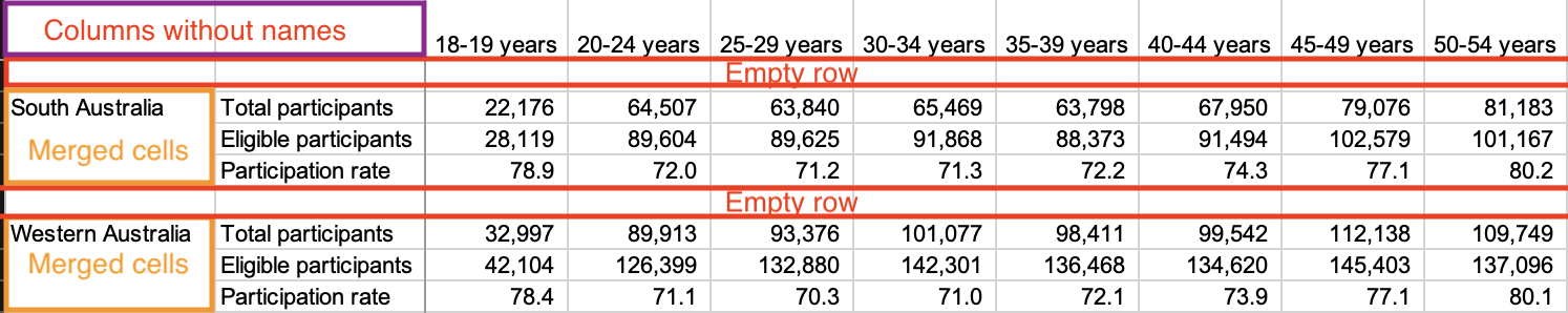
Unfortunately, as can be seen by the annotations we made, these data are not tidy; we show three different issues with the data. This exercise will practice how to bring this dataset into a tidy format so that it can be subject to analysis. The relevant data is available in the tibble abs_partp2017 from the edsdata package.
abs_partp2017## # A tibble: 31 × 17
## ...1 ...2 `18-19 years` `20-24 years` `25-29 years` `30-34 years`
## <chr> <chr> <dbl> <dbl> <dbl> <dbl>
## 1 New South Wales Tota… 109463 296637 295067 307114
## 2 <NA> Elig… 141642 406695 408774 425732
## 3 <NA> Part… 77.3 72.9 72.2 72.1
## 4 <NA> <NA> NA NA NA NA
## 5 Victoria Tota… 83240 249752 256381 265677
## 6 <NA> Elig… 101370 324927 336968 350084
## 7 <NA> Part… 82.1 76.9 76.1 75.9
## 8 <NA> <NA> NA NA NA NA
## 9 Queensland Tota… 61891 175450 175311 182510
## 10 <NA> Elig… 82443 259352 257915 260387
## # ℹ 21 more rows
## # ℹ 11 more variables: `35-39 years` <dbl>, `40-44 years` <dbl>,
## # `45-49 years` <dbl>, `50-54 years` <dbl>, `55-59 years` <dbl>,
## # `60-64 years` <dbl>, `65-69 years` <dbl>, `70-74 years` <dbl>,
## # `75-79 years` <dbl>, `80-84 years` <dbl>, `85 years and over` <dbl>Question 8.1 If the observational unit is the 2017 participation of an Australian age bracket in a territory and we collect 5 measurements per this unit (“Territory/State”, “age group”, “total participants”, “eligible participants”, and “participation rate”), cite at least 2 more violations of the tidy data guidelines. Your answer should note violations other than the missing values caused by the issues raised in the above figure.
-
Question 8.2 Let us first deal with the missing values. These steps can be followed in order:
- The unnamed columns (
...1and...2) should be relabeled to “Territory/State” and “Participation Type”, respectively. - For merged cells, missing values should be filled by looking at the first non-
NAneighbor above, e.g., the second row should take on the value “New South Wales”. - Missing rows should be discarded. This is a reasonable strategy based on what we know about the structure of the data.
The resulting filled-in tibble should be assigned to a name
abs_partp_filled. - The unnamed columns (
Question 8.3 Apply pivot transformation(s) to bring
abs_partp_filledinto tidy format; the resulting tibble after this step should fulfill all tidy data guidelines. Assign this tibble to the nameabs_partp_tidy.Question 8.4 What proportion of results had a participation rate less than 60%?
Question 8.5 Which territory/state had the third smallest eligible voting population in the 18-19 age bracket?
Question 8.6 In the different territories surveyed, what is/are the most frequent age bracket(s) with the lowest participation rates in the survey? Your answer should be expressed as a tibble with two variables named
Age groupandn.
Question 9 This question is a continuation of Question 8. We will now analyze the 2017 Australian Marriage Law Postal Survey another way by looking at the response data. To enrich the analysis, we will overlay the responses with educational qualification data from the 2016 Australian census of population and housing, also released through ABS. We have prepared these data for you, available in the tibbles abs_resp2017 and abs_census2016 from the edsdata package.
abs_resp2017## # A tibble: 8 × 6
## `Territory/State` Yes `Yes (%)` No `No (%)` Total
## <chr> <dbl> <dbl> <dbl> <dbl> <dbl>
## 1 New South Wales 2374362 57.8 1736838 42.2 4111200
## 2 Victoria 2145629 64.9 1161098 35.1 3306727
## 3 Queensland 1487060 60.7 961015 39.3 2448075
## 4 South Australia 592528 62.5 356247 37.5 948775
## 5 Western Australia 801575 63.7 455924 36.3 1257499
## 6 Tasmania 191948 63.6 109655 36.4 301603
## 7 Northern Territory 48686 60.6 31690 39.4 80376
## 8 Australian Capital Territory 175459 74 61520 26 236979
abs_census2016## # A tibble: 64 × 4
## `Education Qualification` `Territory/State` Count `Percent (%)`
## <chr> <chr> <dbl> <dbl>
## 1 Postgraduate Degree Level New South Wales 344490 5.65
## 2 Postgraduate Degree Level Victoria 260039 5.37
## 3 Postgraduate Degree Level Queensland 134242 3.54
## 4 Postgraduate Degree Level South Australia 50993 3.69
## 5 Postgraduate Degree Level Western Australia 76660 3.84
## 6 Postgraduate Degree Level Tasmania 13408 3.19
## 7 Postgraduate Degree Level Northern Territo… 6298 3.51
## 8 Postgraduate Degree Level Australian Capit… 34819 10.8
## 9 Graduate Diploma and Graduate Certifi… New South Wales 103340 1.70
## 10 Graduate Diploma and Graduate Certifi… Victoria 119226 2.46
## # ℹ 54 more rowsNote that these data are at the Territory/State level, while the participation data in Question 8 was broken down further into age brackets.
Question 9.1 Let us explore the relationship between education level and survey response. Using the census data, form a tibble that gives the percentage of Australians that hold at least a bachelor’s degree, i.e., a qualification level that is either “Bachelor Degree Level”, “Graduate Diploma and Graduate Certificate Level”, or “Postgraduate Degree Level.” These designations are based on the Australian Standard Classification of Education (ASCED). The resulting tibble should have two variables,
Territory/StateandAt least Bachelor (%), and be assigned to a namebachelor_by_territory.Question 9.2 Annotate
bachelor_by_territorywith the survey response data by joiningbachelor_by_territorywithabs_resp2017. Assign the resulting joined tibble to the namewith_response.Question 9.3 Note briefly the reason for selecting the join function you used. For instance, if you used
inner_join(), why notleft_join()orright_join()?Question 9.4 Form a subset of
with_responsethat has two rows giving the territory with the highest and lowest support for same-sex couples. Assign this tibble to the namehighest_lowest_support.Question 9.5 According to your findings, does there appear to be an association between survey response and territories with larger percentages of advanced degree holders? Why or why not?
Question 10 Consider the tibbles election and unemp_usda from the edsdata package.
These datasets give county-level results for presidential elections in the USA and the population and unemployment rate of all counties in the US, respectively. The data in election was made available by the MIT Election Data and Science Lab (MEDSL) and contains county-level returns for presidential elections from 2000 to 2020. The data in unemp_usda was prepared by USDA, Economic Research Service and gives county-level socioeconomic indicators for unemployment rates.
An important variable in both datasets is the FIPS code. FIPS codes are numbers which uniquely identify geographic areas. Every county has a unique five-digit FIPS code. For instance, 12086 is the FIPS code that identifies Miami-Dade, Florida.
Question 10.1 Select the relevant unemployment and voting returns data specifically for 2008. The resulting unemployment tibble should contain three columns: FIPS code, state, and the unemployment rate as of 2008. Store these tibbles in the names
election2008andunemp2008.Question 10.2 Some observations in
election2008contain a missing FIPS code. Why might that be?Question 10.3 Locate these rows and then filter them from your
election2008. Assign the resulting tibble back toelection2008.-
Question 10.4 Suppose that we want to create a new tibble that contains both the election results and the unemployment data. More specifically, we would like to add unemployment information to the election data by joining
election2008withunemp2008. Assign the resulting tibble to the nameelection_unemp2008.HINT: What is the key we can use to join these two tables? Note that the column names may be different for the key in each table. For example: we would like to join on the key
student_idbut one table has a columnstudentIDand the otherstudent_id. In the join function we use, we can say???_join(tibble_a, tibble_b, by = c("studentID" = "student_id")). -
Question 10.5 Explain why the join function you selected (e.g., right join, left join, etc.) is appropriate for this problem. Why not choose another join function instead?
Let us explore the relationship between candidate votes and unemployment rate for each state.
-
Question 10.6 Create a tibble from
election_unemp2008that contains, for each state, only the candidate that received the most amount of votes. Assign the resulting tibble to the namestate_candidate_winner2008. It should contain three variables:state,candidate, andvotes. Here is what the first few rows ofstate_candidate_winner2008looks like:state candidate votes ALABAMA JOHN MCCAIN 1266546 ALASKA JOHN MCCAIN 193841 ARIZONA JOHN MCCAIN 1230111 … … … -
Question 10.7 The following tibble
unemp_by_state2008gives an average unemployment rate for each state by averaging the unemployment rate over the respective counties.unemp_by_state2008 <- election_unemp2008 |> group_by(state) |> summarize(avg_unemp_rate = mean(Unemployment_rate_2008, na.rm = TRUE)) unemp_by_state2008Create a new tibble that contains both the candidate winner voting data and the state-level average unemployment data. More specifically, we would like to add the state-level average unemployment data to the winner voting data by joining
state_candidate_winner2008withunemp_by_state2008. Assign the resulting tibble to the namestate_candidate_winner_unemp2008. Question 10.8 Using
state_candidate_winner_unemp2008, generate a tibble that gives the top 10 states with the highest average unemployment rate. Assign this tibble to the nametop_10.
Question 11 At the College of Pluto, the six most popular majors are Astronomy, Biology, Chemistry, Data Science, Economics, and Finances. The applicants to the college specify their preference for a major, and the college selects the student with some criteria. The tibble pluto in the edsdata package gives the selection result from one year.
pluto## # A tibble: 12 × 4
## Major Gender Applied Accepted
## <chr> <chr> <dbl> <dbl>
## 1 Astronomy Male 825 511
## 2 Astronomy Female 168 148
## 3 Biology Male 560 352
## 4 Biology Female 25 17
## 5 Chemistry Male 325 120
## 6 Chemistry Female 593 352
## 7 Data Science Male 417 139
## 8 Data Science Female 375 298
## 9 Economics Male 191 53
## 10 Economics Female 393 240
## 11 Finances Male 373 22
## 12 Finances Female 641 563Question 11.1 Add a new variable
Proportionthat, for each gender, gives the proportion of accepted applicants to some major. Assign the resulting tibble to the namepluto_with_prop.Question 11.2 Which major saw the highest proportion of accepted male applicants? How about accepted woman applicants? Use a
dplyrverb to answer this. Your resulting tibble should have two rows, one for each gender, that gives the corresponding major with the largest proportion of accepted applicants.-
Question 11.3 Using
pluto_with_prop, writedplyrcode that gives the top two majors with the largest gap in acceptance percentage between men and women. The resulting tibble should have two variables: the major and the quantity of the difference.HINT: The function
diff()may be helpful for computing the difference within a group.
Question 12: Examining racial breakdown in the College Scorecard. Section 4.8 presented a case study of how to tidy the College Scorecard dataset. Let us play some more with the dataset. The table is available in the name scorecard_fl from the edsdata package.
scorecard_flWe will be using the variables appearing on relevant_cols.
relevant_cols <- c("INSTNM", "CITY", "ZIP", "UGDS",
                   "NPT4_PUB", "NPT4_PRIV",
                   "UGDS_WHITE", "UGDS_BLACK",
                   "UGDS_HISP", "UGDS_ASIAN", "UGDS_AIAN")
Question 12.1 First, collect the variables appearing only in
mylistand store the data inwith_race. For this action, you can use the dplyr helper functionall_oftogether withselect.Question 12.2 Of the variables we have selected,
UGDSrepresents the total number of enrolled students (as a string). We already know whatNPT4_PUBandNPT4_PRIVrepresent. What doUGDS_WHITEandUGDS_AIANrefer to? Have a look at the glossary and data dictionary to determine what these variables mean.Question 12.3 As in the textbook, we will remove the four-digit route number in
ZIPby replacing the part with the empty string. Call the new variableZIP5and insert it after theCITYvariable. Store the new data frame back in the namewith_race.-
Question 12.4 In the textbook, we looked at generating a Boolean column representing whether or not a college is a private or public institution. We also looked at generating from a string-valued column representing a number to a new column representing a number using
as.double.Let’s perform the following steps:
- Create a new Boolean variable called
publicthat indicates whether or not the college is a public institution, to be added beforeZIP5. - The variables
UGDS,UGDS_WHITE,UGDS_BLACK,UGDS_HISP,UGDS_ASIAN, andUGDS_AIANare currently expressed as strings. Convert these columns to proper numeric columns usingas.double. The operation can be performed in one step by usingacrosswithin themutatecall.
Store the resulting data frame in
with_race. - Create a new Boolean variable called
Question 12.5 By multiplying
UGDSby each of the five ratios, you can calculate the number of students in each of the categories. Call the numbern_XYZwhereXYZrepresents the category, and add the five numbers you can calculate from them afterUGDS. Call the new tibblestudent_counts.Question 12.6 You may observe that the five categories do not cover the entire racial composition. Let’s create a new variable
n_othersby subtracting the five numbers from the total (UGDS). Add it aftern_aian. Call the new tibblestudent_counts_others.-
Question 12.7 Based on what you have calculated, find out which institution has the largest number of …
- Black students?
- Hispanic students?
- Asian students?
You can find the answer by reordering the rows in the descending order of the ethnicity.
Question 12.8 Let us see which 5-digit ZIP code corresponds to the institutions with the largest number of White students. Group by ZIP code and compute the total count of
n_whiteastotal. Then form a single row that contains the ZIP code with the largest number of White students, along with the corresponding count.Question 12.9 Which institution(s) correspond to the ZIP code that you found? Use a
dplyrverb to help you answer this.-
Question 12.10 Let us write a function
examine_by_zipthat accomplishes the task of finding the schools with the highest number of a student group broken down by some ethnicity (e.g.,n_white) with the ZIP code aggregation.This function:
- Receives a parameter representing a variable in
student_counts_others(e.g.,n_white), generates a summarized table, computes the total, and arranges the rows in the descending order of the total, in the same manner as Question 12.8.
- The function then examines the first element of the
ZIP5variable and uses it to obtain the schools whose ZIP matches the ZIP code, in the same manner as Question 12.9.
After writing the function, run it with
examine_by_zip(n_white)to ensure that the result matches the answer you obtained in the previous question.Note: Referencing the variable
column_labelrequires a double curly-bracketing when used within the function. This is an advanceddplyrusage that we will learn more about later. Here is an example usage of the incantation for the purpose of this exercise:embraced <- function(column_label) { student_counts_others |> summarize(mean_num = mean({{ column_label }}, na.rm=TRUE)) } embraced(n_white) embraced(n_others)examine_by_zip <- function(column_label) { } examine_by_zip(n_white) - Receives a parameter representing a variable in