4 Building Simulations

The previous chapters have shown the basics of tidying, transforming, and visualizing data using R and the tidyverse. Armed with these tools, this unit turns to how we can extract insights from our data. Key to this investigation is statistics and inherent to that is the notion of randomness.

We use the word random all the time on a regular basis. For instance, you may be familiar with the concept of gachapon or loot boxes in PC and mobile games which gives players a chance to obtain prized items using real-world currency. While they have recently stirred up much controversy, the basic idea boils down to how to leverage randomness.

We often speak of randomly picking a number between 1 and 100. If someone chooses the number by adding the day of the month plus the minute of the hour showing on the clock of her smart watch, her choice is not random; once you have learned what she has chosen previously, you know what she will choose again. Therefore, anything generated by a systematic, predetermined, and deterministic procedure is not random.

Randomness is so essential to conducting experiments in statistics because it is what allows us to simulate physical processes in the real world, often thousands and hundreds-of-thousands of times. All this at zero cost of coordinating an actual physical experiment, which may not be feasible depending on the circumstances.

This chapter begins by exploring randomness using R. We will then leverage randomness to build out simulations of real life phenomena – like birthdays! – and how we may extract insights from them.

4.1 The `sample` Function

We begin our study by learning how to generate random numbers using R. There are many functions that R has which involve random selection; one of these is called sample(). It picks one item at random from a list (i.e., vector), where the choice will likely occur at all positions. A prime example of randomness is tossing a coin with chance of heads 50% and chance of tails 50%.

fair_coin <- c("heads", "tails")
sample(fair_coin, size = 1)

## [1] "heads"

Run the cell a few times and observe how the output changes. The unpredictable nature makes the code, though short, stand out from all the R code we have written so far.

Note that the function has the form sample(vector_name, size), where vector_name is the name of the vector from which we will select an item and size is how many items we want to select from the vector.

Here is another example: a football game (“American football” for non-US readers) begins each half by kicking a football from the 20-yard line of a team toward the goal of the opponent. The decision of which team gets to kick the ball is through a ritual that takes place three minutes prior to the “kick off”. In the ritual, a referee tosses a coin and the visiting team calls “heads” or “tails”.

If the visiting team calls correctly, the team gets to decide whether the team will kick or receive; otherwise, the home team makes the decision. Note that the ritual is somewhat redundant.

Suppose that the referee throwing the coin is not clairvoyant and has no powers to foretell “heads” or “tails” and that the coin is the same fair coin from our previous example. Then, the referee can simply throw the coin and make the visiting team kick the ball if the coin turns “heads” (or “tails” for what’s its worth).

Thus, the action of choosing the team boils down to selecting from a two-element vector consisting of “kick” and “receive” with chance of 50% for each.

two_groups <- c("kick", "receive")
sample(two_groups, size = 1)

## [1] "receive"

A nice feature of sample is that we can instruct it to repeat its element-choice action multiple times in sequence without influence from the outcome from the previous runs. For instance, we can select the kicking teams for 8 games.

sample(two_groups, size = 8, replace = TRUE)

## [1] "kick"    "receive" "receive" "kick"    "kick"    "receive" "kick"   
## [8] "kick"

Note that a third argument replace is specified here. By setting it to TRUE, we allow the same selection (say, receive) from the two_groups vector to be made more than once. We call this method sampling with replacement. In contrast, toggling this argument to be FALSE would make choices from the previous executions unavailable. We call this way sampling without replacement. R does this by default.

What happens if the size of the vector is smaller than the number of repetitions?

sample(two_groups, size = 8)

There are not enough elements to choose from!

Note that we have made an implicit interpretation of the code: we wrote the code assuming that it will tell the role that the visiting team will play at the kick off; that is, if the value the code generates is kick then the visiting team will kick and if it is receive they will receive. We must not mistake this interpretation. That is, the output the code produces is NOT the role the home team will play; it is for selecting the action of the visiting team. Implicit interpretations we make on the code often play an important role.

If the visiting team is very keen to start by kicking, we may choose to instead translate the outcome as Yes when it is kick and No otherwise. If we choose such a Yes/No interpretation, we view the random scheme producing kick as an “event” and interpret the output being kick as the event “occurring”.

4.2 `if` Conditionals

Often times in programming work we need to take a certain action based on the outcome of an event. For instance, if a coin turns up heads, a friend wins a $5 bet or a visiting team in football is designated as the “kicker”. Such conditional statements and how to use them in programming are the subject for this section.

4.2.1 Remember logical data types?

We saw in an earlier chapter that one of the core data types is logical data. These were the easiest to remember of the bunch because logical data types can only have one of two values: TRUE and FALSE. We also often call such values booleans.

A major use of logical data is to direct computation based on the value of a boolean. In other words, we can write code that has two choices for some part of its action where which of the two actions actually occurs depends on the value of the boolean.

If we draw the choice-inducing boolean value from random generation, say using sample, we can randomly select among possible actions. We call such an “action selection” based on the value of a boolean conditional execution.

4.2.2 The `if` statement

A program unit in a conditional execution is a conditional statement. A conditional statement is one that allows selection of an action from multiple possibilities. In R and in many other languages, we usually write a conditional statement as a multi-line statement. It is entirely possible to put everything in one, but such style is confusing and prone to errors.

Conditional statements usually reside inside a function. This allows us to express alternative behavior depending on argument values.

In R, and in many programming languages, a conditional statement begins with an if header. What appears after the keyword is a pair of parentheses, in which a condition to examine appears. After the condition part appears an action to perform, which is a series of statements flanked by a pair of curly braces.

The syntax specifies that if the condition inside the pair of parentheses is true, the program executes the statements appearing in the ensuing pair of braces. We call a statement in this form an if statement.

Let us see our first example of an if statement, which is a function that returns the sign of a number.

sign <- function(x) {
  if (x > 0) {
    return("positive")
  }
}
sign(3)

## [1] "positive"

The function sign receives a number and returns a string representing the sign of the number. Actually, the return value of the function exists only if the number is strictly positive; otherwise, the function does not return anything.

print(sign(-3))

## NULL

What is the boundary separating positive and nothing? We know that the condition is x > 0 so we can say that the boundary is the point 0, but 0 falls on the side that produces no return.

Can we make the return positive when x is equal 0? Sure can!

sign <- function(x) {
  if (x >= 0) {
    return("positive")
  }
}
sign(0)

## [1] "positive"

sign(0.1)

## [1] "positive"

print(sign(-0.1))  # force a print

## NULL

We can put a series of conditional statements in a function. If a conditional statement contains a return statement and R executes that statement, R skips the remainder of the code in the function.

sign <- function(x) {
  if (x > 0) {
    return("positive")
  }
  if (x < 0) {
    return("negative")
  }
}
sign(2)

## [1] "positive"

sign(-2)

## [1] "negative"

print(sign(0))  # force a print

## NULL

Instead of saying “if x is less than 0, it is negative”, it would be more natural to say “otherwise, if x is less than 0, it is negative”. We can express “otherwise” using the keyword else. Let’s revise the above code.

sign <- function(x) {
  if (x > 0) {
    return("positive")
  } else if (x < 0) {
    return("negative")
  }
}
sign(3)

## [1] "positive"

sign(-3)

## [1] "negative"

print(sign(0))  # force a print

## NULL

What do we do about 0? By adding another else if block to the code, we can make the function return something in the case when the number is 0.

sign <- function(x) {
  if (x > 0) {
    return("positive")
  } else if (x < 0) {
    return("negative")
  } else if (x == 0) {
    return("neither positive nor negative")
  }
}

sign(0)

## [1] "neither positive nor negative"

Since the condition x == 0 is exactly the condition x satisfies when the execution reaches the second else if block, we can jettison the if and the condition. The resulting block is what we call an else block.

sign <- function(x) {
  if (x > 0) {
    return("positive")
  } else if (x < 0) {
    return("negative")
  } else {
    return("neither positive nor negative")
  }
}

sign(0)

## [1] "neither positive nor negative"

4.2.3 The `if` statement: a general description

We are now ready to present a more general form of the if statement.

if (<expression>) {
    <body>
} else if (<expression>) {
    <body>
} else if (<expression>) {
    <body>
...
} else {
    <body>
}

The keyword else means “otherwise” and the keyword else if is a combination of else and if. We can stack up else if blocks after an initial if to define a series of alternative options.

Following are some notes to keep in mind:

An if-block cannot begin with an else in the series.
There must exist one if clause.
When a series of else if blocks appear after an if, this represents a series of alternatives. We call this an if sequence.
An if without a preceding else begins a new if sequence.
R scans all the conditions appearing in an if sequence takes an action when it finds a condition that evaluates to TRUE. All other actions before and after the matching one are ignored.
The else block is optional; it takes care of everything that does not have a match.

4.2.4 One more example: comparing strings

We end this section with another example, this time comparing strings.

get_capital <- function(x) {
  if (x == "Florida") {
    return("Talahassee")
  } else if (x == "Georgia") {
    return("Atlanta")
  } else if (x == "Alabama") {
    return("Montgomery")
  } else {
    return("Oops, don't know where that is")
  }
}

Here is a dataset containing some students and their state of residence.

some_students <- tibble(
  name = c("Xiao", "Renji", "Timmy", "Christina"), 
  state = c("Florida", "Florida", "Alabama", "California")
)
some_students

## # A tibble: 4 × 2
##   name      state     
##   <chr>     <chr>     
## 1 Xiao      Florida   
## 2 Renji     Florida   
## 3 Timmy     Alabama   
## 4 Christina California

We can annotate the tibble with a new column containing the capital information for each state using a purrr map.

some_students |>
  mutate(capitol = map_chr(state, get_capital))

## # A tibble: 4 × 3
##   name      state      capitol                       
##   <chr>     <chr>      <chr>                         
## 1 Xiao      Florida    Talahassee                    
## 2 Renji     Florida    Talahassee                    
## 3 Timmy     Alabama    Montgomery                    
## 4 Christina California Oops, don't know where that is

Note how Christina’s capital information defaults to the result of the else condition.

4.3 `for` Loops

Let us now use conditional execution to simulate a simple betting game on a coin.

4.3.1 Prerequisites

We will need some functions from the tidyverse in this section, so let us load it in.

library(tidyverse)

4.3.2 Feeling lucky

We will use the same fair coin from the kick-off we saw in the football example. However, feeling lucky, you wager that you can make some money off this coin by betting a few dollars on heads – can we tell if your intuition is right? Let’s find out!

We imagine a function that will receive a string argument representing the side the coin is showing, and returns the result of the bet. If the coin shows up heads you get 2 dollars. But, if it shows tails you lose 1 dollar.

one_flip <- function(x) {
  if (x == "heads") {
    return(2)
  } else if (x == "tails") {
    return(-1)
  } 
}

Let us see how the function works.

c(one_flip("heads"), one_flip("tails"))

## [1]  2 -1

To play the game based on one flip of a coin, we can use sample again.

sides <- c("heads","tails")
one_flip(sample(sides, size = 1))

## [1] 2

We can avoid having to create a sides variable by including the vector directly as an argument.

one_flip(sample(c("heads","tails"), size = 1))

## [1] 2

Now let us expand this and develop a multi-round betting game.

4.3.3 A multi-round betting game

Previously, we split the game into two actions: a function one_flip computing the gain/loss and a sample call simulating one round of the game using the gain/loss function. We now combine these two into one.

betting_one_round <- function() {
  # Net gain on one bet
  x <- sample(c("heads","tails"), size = 1) 
  if (x == "heads") {
    return(2)
  } else if (x == "tails") {
    return(-1)
  } 
}

Betting on one round is easy – just call the function!

betting_one_round()

## [1] 2

Run the cell several times and observe how the value is sometimes 2 and sometimes -1. How often do we get to see 2 and how often do we get to see -1? Will your wager come out on top?

You could run this function multiple times and tally, of the runs you observed, how many times you won 2 dollars and how many times you lost a dollar. You could then compare the difference between the gains and losses. This is quite a tedious process and we still don’t have a sense of how variable the results are. For that, we would need to run this process thousands or millions of times. Should we grab a good pencil and get tallying? No way! Let’s use the power of R.

We can instruct R to take care of the repetitive work by repeating some action a number of times with specific instruction such as, “for round X, use this information”. Iteration is the name we use in programming to refer to things that repeat. In R and in many other languages, a keyword that leads a code in iteration is for. We also use the word loop to refer to a process that repeats.

So a code that repeats a process with for as the header is a for-loop.

In R, the way to specify a for-loop is to say: “for each item appearing in the following sequence, starting from the first and towards its end, do this.”

for (hand in c("rock", "paper", "scissors")) {
  print(hand)
}

## [1] "rock"
## [1] "paper"
## [1] "scissors"

for (season in c("spring", "summer", "fall", "winter")) {
  print(season)
}

## [1] "spring"
## [1] "summer"
## [1] "fall"
## [1] "winter"

In the two for loops, hand and season are the names we use to refer to the elements that the iteration picks from the lists. In other words, the first for-loop picks an item from the three-element sequence and we use the name hand to access the item. The same is true for the second for-loop.

Our present interest is in writing a program that repeats the betting game many times. To repeat an action a number of times, we use a pair of numbers with a colon in between. The expression is X:Y, where X represents the start and Y the end. The expression represents the series of integers starting from X and ending with Y.

1:5

## [1] 1 2 3 4 5

30:20

##  [1] 30 29 28 27 26 25 24 23 22 21 20

a <- 18
b <-  7
a:b

##  [1] 18 17 16 15 14 13 12 11 10  9  8  7

b:a

##  [1]  7  8  9 10 11 12 13 14 15 16 17 18

Wow! R is so smart that when the second number is smaller than the first number, it decreases the number by 1, instead of increasing it by 1.

Now we can use the sequence generation to write a for-loop. This one prints 1 through 5.

for (i in 1:5) {
  print(i)
}

## [1] 1
## [1] 2
## [1] 3
## [1] 4
## [1] 5

We can apply this to the betting game.

for (i in 1:10) {
  print(betting_one_round())
}

## [1] 2
## [1] -1
## [1] -1
## [1] -1
## [1] -1
## [1] 2
## [1] -1
## [1] -1
## [1] -1
## [1] 2

Note that the function better_one_round is self-contained, meaning not requiring an argument, and so the code that R runs is identical among the ten iterations. However, betting_one_round has a call to sample and that introduces randomness in the execution and, therefore, the results we see in the ten lines are not uniform and can be different each time we run the for loop.

4.3.4 Recording outcomes

You may have realized “the results of the ten runs disappear each time I run it; is there a way to record them?” The answer: yes!

We create an integer vector to store the results, where the vector has the same length as the number of times we issue a bet; each element in the vector stores the result of one bet.

rounds <- 10
outcomes <- vector("integer", rounds)
for (i in 1:rounds) {
  outcomes[i] <- betting_one_round()
}

outcomes

##  [1]  2  2  2 -1 -1  2 -1 -1  2  2

This will do the job. The body of this for loop contains two actions: (1) run the betting function betting_one_round(), and (2) store the result into ith slot of the outcomes vector. Both actions are executed for each item in the sequence 1:rounds.

You may have noticed how stepping through the outcomes vector this way, individually assigning each element the result of one bet, can be cumbersome to write. If so, you would be in good company. The philosophy of R, and especially the tidyverse, prefers to eliminate the need to write many common for loops. We saw one example of this already when we used map from the purrr package to apply a function to a column of data. Here, we will use the function replicate to repeat a simulation many times.

Here is how we can rewrite our simulation using just two lines of code.

rounds <- 10
outcomes <- replicate(n = 10, betting_one_round())

outcomes

##  [1]  2 -1 -1 -1 -1  2  2 -1  2 -1

We can use sum to count the number of times money changed hands.

sum(outcomes)

## [1] 2

Looks like we made some money!

Note that while replicate eliminates the need to write for loops in common situations, R internally must still perform a for loop, i.e., the code for replicate contains a for loop and it is not directly visible to us as the programmer who wrote the code. Therefore, the chief benefit of using constructs like replicate and map is not for its speed, but clarity: it is much easier to read (and write!).

If you are still not convinced, we defer to a prominent data scientist and an authority on tidyverse for an explanation.

Of course, someone has to write loops. It doesn’t have to be you. — Jenny Bryan

4.3.5 Example: 1,000 tosses

Iteration using replicate is a handy technique. For example, we can see the variation in the results of 1,000 bets by running exactly the same code for 1,000 bets instead of ten.

rounds <- 1000
outcomes <- replicate(n = rounds, betting_one_round())

The vector outcomes contains the results of all 1000 bets.

length(outcomes)

## [1] 1000

How much money did we make?

sum(outcomes)

## [1] 536

To see how often the two different possible results appeared, we can create a tibble from outcomes and then use ggplot2.

outcome_df <- tibble(outcomes)
ggplot(outcome_df, aes(x = outcomes)) + 
  geom_bar() + 
  coord_flip()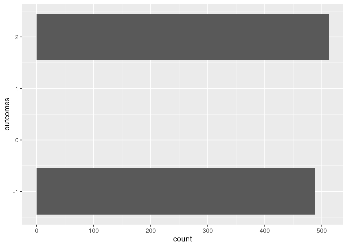

As we would expect, each of the two outcomes 2 and -1 appeared about 500 of the 1000 times. And, because we bet an extra dollar for every heads we get, we come out on top. Not bad!

4.4 A Recipe for Simulation

Simulation, in data science, refers to the use of programming to imitate a physical process. Sometimes we call it “computer simulation” to articulate that the a computer is the author of such simulation. A simulation consists of three main steps.

4.4.1 Prerequisites

As before, let us load in the tidyverse.

library(tidyverse)

4.4.2 Step 1: Determine what to simulate

The first step is to figure out which part of the physical process we want to imitate using computation and decide how we will represent that part numerically.

4.4.3 Step 2: Figure out how to simulate one value

The second step is to figure out how to generate values for the numerical representation from the first step using a computer program. If some numbers require updating during the simulation procedure, we will figure out how to update them. Randomness is often a key ingredient in this step. This is usually the most difficult part of the simulation to complete.

4.4.4 Step 3: Run the simulation and visualize!

The fourth step is to run the simulation and develop insights from the result, often using visualization. During this step we also must decide the number of times to simulate the quantity from the second step. To get a sense of how variable a quantity is, we must run step 2 a large number of times. We saw that in the previous section with simulating bet wins/losses we ran the experiment 1,000 times. But we may need to run a simulation even more, say hundreds of thousands or millions of times.

4.4.5 Putting the steps together in R

Note that we have followed these same steps in the betting experiment from the previous section. We can write the steps more generally here:

Create a “rounds” variable, that is, an integer containing the number of desired repetitions.
Create an “experiment” function to simulate one value based on the code we developed.
Call the function replicate to replicate the experiment function a great number of times.
- Store the results to a variable. We call this the “outcomes” vector.
- A general format takes the form: outcomes <- replicate(n = rounds, experiment_func())

The outcomes vector will contain all the simulated values. A good next step would be to visualize the distribution of the simulated values by counting the number of simulated values that fall into some category or, perhaps more directly, by using ggplot!

We now turn to some examples.

4.4.6 Difference in the number of heads and tails in 100 coin tosses

Let us return to the coin tosses. As we see powers of 10 as the easiest kind of numbers to deal with, let us back down from 300 to 100. If the coin is fair, we anticipate a half of the tosses we make is “Head”. The simulation we have written receives as the number of repetitions, and returns a vector representing the results of the simulated coin tosses with an added interpretation of “heads” as 1 and “tails” as -1. We can go back to the process of flipping a coin and develop an insight as to when we flip a coin 300 times, how the number of “heads” is likely to look.

In this example we will simulate the number of heads in 300 tosses of a coin. The histogram of our results will give us some insight into how many heads are likely.

Let’s get started on the simulation, following the steps above.

4.4.7 Step 1: Determine what to simulate

We want to simulate the process of tossing 300 fair coins, where each coin toss generates “heads” or “tails” as the outcome. There is only one number we are interested in the physical process - the number of “heads”.

4.4.8 Step 2: Figure out how to simulate one value

Now we know that we want to know the number of “heads” in 100 coin tosses, we have to figure out how to make one set of 100 tosses and count the number of heads. Let’s start by creating a coin. We eliminate the gain/loss calculation from the previous program in the ensuing simulation program. We start by stating the two possible outcomes of toss. What we define is a two-element vector, as before, and we call it sides.

sides <- c("heads", "tails")

We use sample() to sample from the two-element vector. Recall that we can specify the number of samples and if we want to replenish the vector with the item that the sample has chosen. The code below shows how we sample from sides 8 times with replacement.

tosses <- sample(sides, size = 8, replace = TRUE)
tosses

## [1] "tails" "tails" "heads" "tails" "tails" "tails" "tails" "tails"

We can count the number of heads by using sum() as before:

sum(tosses == "heads")

## [1] 1

Our goal is to simulate the number of heads in 100 tosses. We have only to replace the 8 with 100.

outcomes <- sample(sides, size = 100, replace = TRUE)
num_heads <- sum(outcomes == "heads")
num_heads

## [1] 48

Play with the code a few times to see how close the number gets to the expected one half, 150.

one_trial <- function() {
  outcomes <- sample(sides, size = 100, replace = TRUE)
  num_heads <- sum(outcomes == "heads")
  return(num_heads)
}

You can simply call this function to generate an outcome of one experiment.

one_trial()

## [1] 55

4.4.9 Step 3: Run and visualize!

Here we face a critical question, “for our goal of developing an insight about coin tosses, how many times do we want to repeat it?” We can easily run the code 10,000 times, so let’s choose 10,000 times.

We have programmed one_trial so that it executes 100 coin tosses and returns the number of “Heads”. We now need a loop to repeat one_trial as many times we want.

To do that, we use the replicate construct.

# Number of repetitions
num_repetitions <- 10000

# simulate the experiment!
heads <- replicate(n = num_repetitions, one_trial())

By executing heads after this produces all elements of heads. That will be a lot of lines on the screen, so you may not want to do it! Instead, we can ask heads how many elements it has, using the length function we have seen before.

length(heads)

## [1] 10000

Aha! It has the desired number of elements. We can peek at some of the elements in the vector.

heads[1]

## [1] 51

heads[2]

## [1] 52

Using tibble we can collect the results as a table. Recall that tibble needs the index values and the data.

results <- tibble(
  repetition = 1:num_repetitions,
  num_heads = heads
)

results

## # A tibble: 10,000 × 2
##    repetition num_heads
##         <int>     <int>
##  1          1        51
##  2          2        52
##  3          3        53
##  4          4        48
##  5          5        44
##  6          6        46
##  7          7        46
##  8          8        57
##  9          9        51
## 10         10        54
## # … with 9,990 more rows

ggplot(results) + 
  geom_histogram(aes(x = num_heads, y = after_stat(density)), 
                 color = "gray", fill = "darkcyan", 
                 breaks = seq(30.5, 69.6, 1))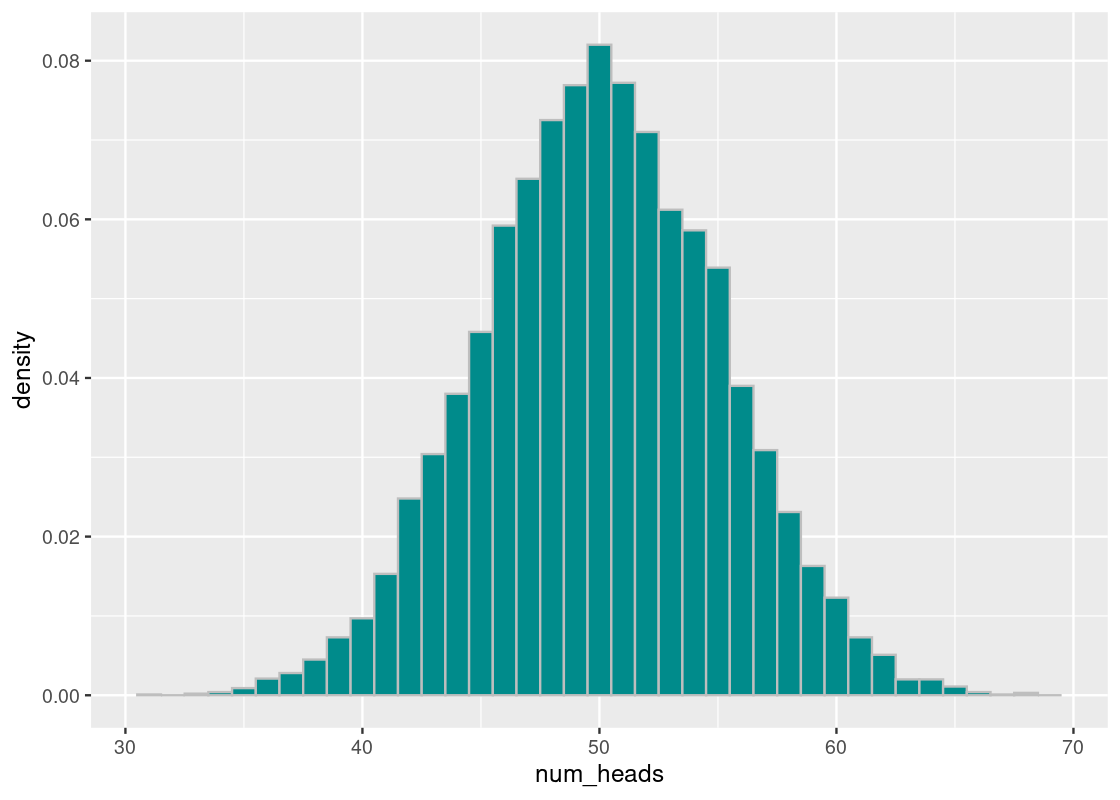

In this histogram, each bin has width 1 and we place it centered on the value. For example, the vertical bar on 50 is the number of times the simulation generated 50 as the result. We see that the histogram looks symmetric with 50 as the center, which is a good sign. Why? Our expectation is that the number 50 is the ideal number of “Heads” in 100 tosses of a fair coin. If the coin is fair, for all number $d$, the event that we see $50-d$ “Heads” is as likely to happen as the event that we see $50+d$ Heads. The symmetry that we observe confirms the hypothesis. We also see that about 8% (i.e., 0.08 on the y-axis) of the simulation results produced 50. Furthermore, we see that very few times we see occurrences of numbers less than 35 or greater than 65. We thus conclude from the experiment that the range of the number is likely to reside in the range $[35,65]$.

4.4.10 Not-so-doubling rewards

There is a famous story of a king awarding a minister with doubling amount of grains. There are many versions of the story, but the gist is like this: one day a king has decided to award a minister for his great work.

The kind asks, “Great work, what do you want from me as a reward? You name it, I will make your wish come true.”
The minister says, “Your Majestry, what an honor! If you are so kind as to indulge me, may I ask to receive grains of rice on a board of chess. We will start with one grain on a space on the board, given one day. The next day, I would like two grains on the next space. The following day, I would like four grains on the third space. Each day, I would like twice as many grains as you have given me on the previous day. In this manner, for the next 64 days, you would be so generous to give me grains of rice. Would that be too imposing to ask?”
The king says, “You ask so little. That would be so easy to do. Of course, this great King will grant you your request.”

The question is how many grains of rice will the minister receive at the end of the 64 day period?

We know the answer to the question. The daily amount doubles each day starting from 1. He would thus receive:

\[ 1 + 2 + 4 + 8 + 16 + \cdots = 2^0 + 2^1 + 2^2 + 2^3 + 2^4 + \cdots+ 2^{63} \]

We can express this quantity more compactly as $2^{64} - 1$.

Why? Suppose he has one more grain in his pocket to add to the piles at the end of the 64th day. We have

\[ 1 + 1 + 2 + 4 + 8 + \cdots + 2^{63} - 1 \]

as the same total amount. The first two occurrences of 1 are equal to 2. So we can simplify the sum as

\[ 2 + 2 + 4 + 8 + \cdots + 2^{63} - 1 \]

We have got rid of the twos. By joining the first two 2’s, we get

\[ 4 + 4 + 8 + \cdots + 2^{63} - 1 \]

At the end of calculation, we get

\[ 2^{63} + 2^{63} - 1 \]

and this is equal to $2^{64}-1$, which is, by the way, an obscenely large number.

We know the story as a fable that tells us we must think before promising something. This story took place hundreds of years ago, where there were no computers. For the king to provide the grains he had promised to give to the minister, he would have ordered a clerk to do the calculation.

If the clerk is super-human, her calculation would be perfect, and so the total amount she would provide would be exactly what we had anticipated. But, since she is human, she is prone to error. In the process of writing down numbers, there may be various errors, such as skipping a digit or writing a wrong digit.

If she does not notice an error, the minister would get a different amount of grains at the end of the 64 days. Suppose we want to mimic the process of her calculation using a computer, with the chance factor in mind. This is how “randomness” comes in to play.

Let us consider two different scenarios for the source of error:

The errors are independent. That is, the error the clerk makes on a day does not affect the bookkeeping the next day.
The errors are dependent. That is, the error the clerk makes affects the next day’s counting and has a lasting effect on the bookkeeping for the remaining days.

The first scenario is easier, so we will develop a simulation scheme for this first. Also, to simplify the number crunching, we consider the number of grains the minister receives at the end of 10th day. We know that this number should equal $2^{10} - 1$.

4.4.10.1 Step 1: Determine what to simulate

We are interested in simulating the number of grains the minister receives at the end of the 10th day, assuming independent errors in bookkeeping. We hypothesize that the number of grains should cluster around $2^{10} - 1 = 1023$.

4.4.10.2 Step 2: Figure out how to simulate one value

We imagine the variability in the clerk’s calculation for the number of grains a minister receives. Based on what we know from the story, three actions are possible:

The clerk counts one less grain.
The clerk counts the right amount of grains.
The clerk counts one extra grain.

We will assume that “getting it right” has a slightly higher chance of occurring ($2/4$) with the other two actions having an equal chance of occurring ($1/4$). We can simulate the clerk’s action using sample and setting the prob argument.

sample(c(-1, 0, 1), 1, prob=c(1/4, 2/4, 1/4))

## [1] 0

The following function receives a number of grains as an argument and returns the number of grains after the clerk’s calculation. This is the amount the minister would receive after some day.

after_clerk_calculation <- function(grains) {
  grains + sample(c(-1, 0, 1), 1, prob=c(1/4, 2/4, 1/4))
}

We can try the function with some arbitrary number of grains, say, 10.

after_clerk_calculation(10)

## [1] 10

Try running this a few times to observe the different outcomes. Sometimes the clerk gets it right (10), counts one less (9), or counts one more (11).

The expected amount the minister should receive each day follows the form $2^{\text{ day number} - 1}$. We can write the following sequence for the amounts starting at day 1 and ending after day 10.

2 ** (0:9)

##  [1]   1   2   4   8  16  32  64 128 256 512

Using a purrr map, we can simulate the amounts after the clerk’s calculation by applying the function after_clerk_calculation to each of the elements in the above sequence.

map_dbl(2 ** (0:9), after_clerk_calculation)

##  [1]   1   3   5   8  15  31  64 127 256 513

Therefore, the total number of grains the minister receives is the sum of these amounts.

map_dbl(2 ** (0:9), after_clerk_calculation) |>
  sum()

## [1] 1023

We now have enough machinery to write a function for simulating one value. This functions receives the number of days as an argument and returns the total grains received by the minister after the given number of days is over.

total_grains_received <- function(num_days) {
  map_dbl(2 ** (0:(num_days - 1)), after_clerk_calculation) |> 
    sum()
}

For a 10-day scheme, we call the function as follows.

total_grains_received(10)

## [1] 1021

Run the cell a few times and observe the variability in the number of grains.

4.4.10.3 Step 3: Run and visualize!

We will use 10,000 repetitions of the simulation this time to get a sense of the variability. Each element of the grains vector stores the resulting number of grains at the end of the 10th day in each simulation of the story.

# Number of repetitions
num_repetitions <- 10000

# simulate the experiment!
grains <- replicate(n = num_repetitions, total_grains_received(10))

As before, we collect our results into a tibble.

results <- tibble(
  repetition = 1:num_repetitions,
  num_grains = grains
)
results

## # A tibble: 10,000 × 2
##    repetition num_grains
##         <int>      <dbl>
##  1          1       1022
##  2          2       1023
##  3          3       1019
##  4          4       1022
##  5          5       1021
##  6          6       1022
##  7          7       1023
##  8          8       1023
##  9          9       1021
## 10         10       1022
## # … with 9,990 more rows

Finally, we visualize our results.

ggplot(results) + 
  geom_histogram(aes(x = num_grains, y = after_stat(density)), 
                 color = "gray", fill = "darkcyan", bins = 18) + 
  geom_point(aes(x = 1023, y = 0), color = "salmon", size = 3)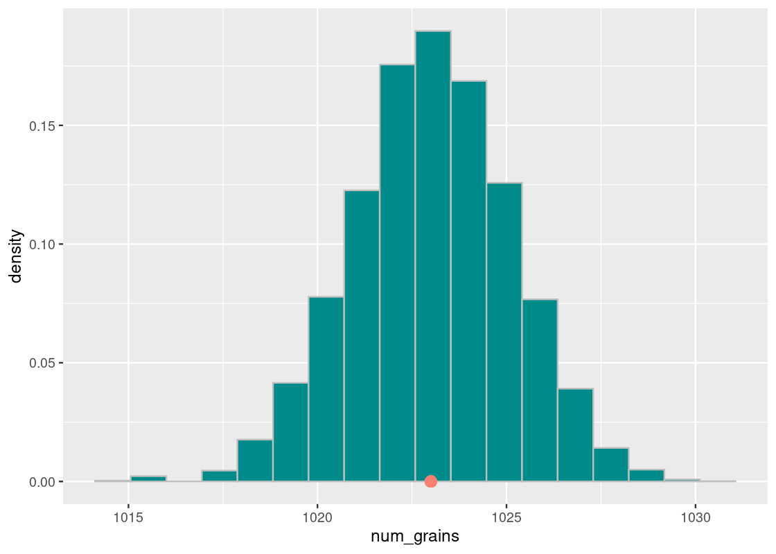

We observe that the number of grains cluster around 1023, as expected (see the orange dot). In general, each round after the first can create a difference of at most 1, so with $N$ rounds, the difference is at most $N - 1$. Our simulation confirms this fact.

4.4.11 Accumulation

We now turn to the second scenario in the doubling grains story. Because the calculation for the next day depends on what happened the previous day, we will not be able to use the map or replicate operations as we did when assuming the errors were independent. We need a programming construct that allows us to update some value as we go along. We could use the for loop construct shown in Section 6.3 to achieve this work easily, but we would like to eliminate the need to write a loop as much as possible.

purrr offers another construct called accumulate that sequentially applies a 2-argument function to elements of a vector. A key aspect of its operation is that each application of the function uses the result of the previous application as the first argument.

Let’s see an example. Consider the following character vector of fruits.

delicious_fruits <- c("apple", "banana", "pineapple", "mango")

We can use accumulate to implement string concatenation. Here, we provide an anonymous function that receives two arguments acc (an accumulator) and nxt (the next element in the input vector). The str_c function is called using the two arguments using the colon as a separator. The effect achieved is the joining, or “concatenation”, of all strings in the vector delicious_fruits into a single string.

accumulate(delicious_fruits, \(acc, nxt) str_c(acc, nxt, sep = ":"))

## [1] "apple"                        "apple:banana"                
## [3] "apple:banana:pineapple"       "apple:banana:pineapple:mango"

There is a good deal of technical detail here so let us unpack what we just did. The accumulator (stored in the argument acc) stores the resulting string after concatenation with each element in the vector delicious_fruits. The accumulation begins with the first element, the string "apple". After concatenation with the argument nxt ( containing the string "banana"), the resulting string is "apple:banana" and the accumulator is updated with this value in the next step of the iteration, available in the argument acc.

The process continues until each element of the input vector has been exhausted. The result of the accumulation at each step is shown in the vector returned by the accumulate function. This vector has the same length as the input vector and the final result appears at the last index (index 4), a single string containing each fruit separated by a colon.

We could discard the intermediate results and extract just the final product by applying the function last from dplyr. Observe how this is equivalent to str_c when used with the collapse setting.

# str_c from stringr with collapse
str_c(delicious_fruits, collapse = ":")

## [1] "apple:banana:pineapple:mango"

# using accumulate!
accumulate(delicious_fruits, \(acc, nxt) str_c(acc, nxt, sep = ":")) |>
  last()

## [1] "apple:banana:pineapple:mango"

We can also set an initial value to use to begin the accumulation.

accumulate(delicious_fruits, \(acc, nxt) str_c(acc, nxt, sep = ":"), 
           .init = "a")

## [1] "a"                              "a:apple"                       
## [3] "a:apple:banana"                 "a:apple:banana:pineapple"      
## [5] "a:apple:banana:pineapple:mango"

This has the effect of extending the resulting vector length by 1.

In some cases, it is desirable to use the accumulator and ignore the elements in the input vector given (in the argument nxt). This can be useful when you care only about the accumulation and repeating this for some number of steps.

For instance, the following accumulate continuously adds 10 to an initial value 10. The length of the input vector controls the number of steps taken, but the vector contents are ignored.

accumulate(541:546, \(acc, nxt) acc + 10, .init = 10)

## [1] 10 20 30 40 50 60 70

It is also possible to terminate the accumulation early based on some condition being met using the done sentinel. This can also be useful depending on the simulation scheme. Question 4 from the exercise set explores this feature in greater depth.

Pop quiz: In the above accumulate example, would you expect the resulting vector to change if we had used the sequence 1:6 as the input vector? Why or why not?

4.4.12 Lasting effects of errors

We can use the accumulate construct in the doubling grains simulation. Recall that, under the second scenario, the error the clerk makes on some day affects the bookkeeping for the remaining days. That is, the amount the clerk gives on a day after the initial day is two times the amount she gave in the previous with a possible error of $\pm$ 1 grain.

We write a function grains_after_day that receives a single argument containing the current number of grains. It returns the sum of the current grains and the calculated grains after after_clerk_calculation is called. When things go right, this has the desired effect of doubling the current number of grains.

grains_after_day <- function(current_grains) {
  new_amount <- current_grains + after_clerk_calculation(current_grains)
  return(max(1, new_amount))
}

The second line is added as a sanity check to ensure the resulting grain amounts do not ever go negative.

We can use this function within an accumulate call to simulate one value in this experiment. Here we provide an initial value 1 to begin the accumulation with and use the input vector only to step the simulation 10 times.

accumulate(1:10, \(acc, nxt) grains_after_day(acc), .init = 1)

##  [1]   1   2   3   6  11  23  47  94 188 375 749

We rewrite the function total_grains_received to use the accumulate call and retrieve the final value.

total_grains_received <- function(num_days) {
  accumulate(1:10, \(acc, nxt) grains_after_day(acc), .init = 1) |> 
    last()
}

We can now call this function a large number of times, say, 10,000, to gauge the amount of variability. Each element of the grains vector stores the resulting number of grains after the 10th day, assuming dependent errors.

num_repetitions <- 10000
grains <- replicate(n = num_repetitions, total_grains_received(10))

Finally, we visualize the result.

grains |>
  tibble() |> 
  ggplot() + 
  geom_histogram(aes(x = grains, y = after_stat(density)), 
                 bins = 18, color = "gray", fill = "darkcyan") +
  geom_point(aes(x = 1023, y = 0), color = "salmon", size = 3)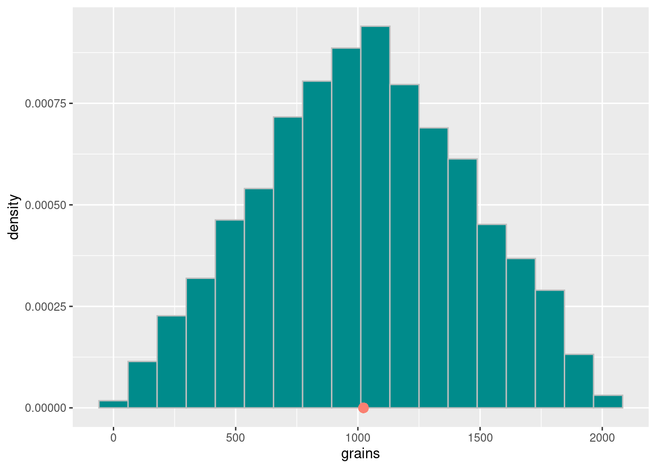

Sometimes the minister received few to no grains at the end of the 10th day and sometimes he received much more than he asked for! Like the first scenario, we see the simulated values cluster again around the expected amount.

4.4.13 Simulation round-up

This section discussed multiple iteration constructs for building simulations. The following list clarifies when to use each.

map_*
- Arguments: (1) a sequence (2) a function that receives as an argument an element from that sequence
- Returns: List or vector the same length as the input sequence
- When to use? Applying a function to a sequence or a tibble column
replicate
- Arguments: (1) Number of repetitions (reps) (2) a function to repeat
- Returns: Vector of length reps that can be stored for later analysis
- When to use? Repeating a function some fixed number of times
accumulate
- Arguments: (1) a sequence (2) a two-argument function; first argument is an accumulator and the second argument an element from the sequence
- Returns: Vector the same length as the input sequence that contains the results of the accumulation at each step (or one longer if .init argument is set)
- When to use? Applying a function where some value needs to be updated through the duration of the simulation

4.5 The Birthday Paradox

Happy birthday! Someone in your class has a birthday today! Or, should we say happy birthdays?

The Birthday Paradox states that if 23 students are in a class, the chances are 50/50 that there are two students among the 23 who have the same birthday. There are 365 days in a year. How is it possible that among just 23 students, we can find two of them that have the same birthday?

4.5.1 Prerequisites

As before, let us load in the tidyverse.

library(tidyverse)

4.5.2 A quick theoretical exploration

We answer the question first by analysis.

Assume that we will consider only a non-leap year (no February 29th – sorry leap year babies!) and each of the 365 birthdays are likely to occur. Since each birthday is likely to occur as any other birthday, we can look at the question at hand by counting the number of possible birthday combinations.

We have 23 students in the class. Each student gets to choose her birthday freely without considering the birthdays of the other 22 students. The 23 students make their choices and then check whether the choices fall into one of the no-duplicate selections.

With no restriction, the number of possible choices of birthdays for the 23 students is

\[ 365 * 365 * 365 * \dots * 365 = 365^{23} \]

These possibilities contain the cases where birthdays may be shared among the people.

In comparison, the number of possibilities for selecting 23 birthdays so that no two are equal to each other requires a bit complicated analysis. We can view the counting problem using the following hypothetical process.

The 23 students in the class will pick their birthdays in order so that there will be no duplicates.

The first student has complete freedom in her choice. She chooses one from the 365 possibilities.
The next student has almost complete freedom. She can pick any birthday but the one the first student has chosen. There are now 364 possibilities.
The third student has again almost complete freedom. She can pick any birthday but the ones the first two students have chosen. Since the first two students picked different birthdays, there are 363 possibilities for the third student.

We can generalize the action. The $k$-th person has $365 - k + 1$ choices.

By combining all of these for the 23 students, we have that the number of possibilities for choosing all-distinct birthdays is

\[ 365 \cdot 364 \cdot 363 \cdot \cdots \cdot 353. \]

Thus, the chances for the 23 students to make the selections so there are no duplicates are thus

\[ (365 \cdot 364 \cdot 363 \cdot \cdots \cdot 343) / 365^{23}. \]

Moving terms, we get that the chances are

\[ \frac{365}{365} \cdot \frac{364}{365} \cdots \frac{343}{365}. \]

The quantity is approximately $0.4927$. The chances we find a duplicate are 1 minus this quantity, which is approximately $0.5073$. Pretty interesting, isn’t it?

4.5.3 Simulating the paradox

The second method, an alternative to the formal mathematical analysis, is to use simulation to mimic the process of selecting 23 birthdays independently from each other. This simulation is slightly more difficult than the ones we have seen in the previous section.

4.5.4 Step 1: Determine what to simulate

In this simulation, we are interested in obtaining the chance or probability that two students in the class have the same birthday among a group of 23 individuals.

4.5.5 Step 2: Figure out how to simulate one value

We start by using sample to draw 23 random birthdays. The vector represented by the sequence 1:365 contains the days in the year one can pick from.

chosen_birthdays <- sample(1:365, size=23, replace=TRUE)
chosen_birthdays

##  [1] 282  51 118  33  86 197 166 289  57 193 179 271 288  59 255  38 352  45  52
## [20] 290 333 128 242

We now check how many duplicates there are in the class.

sum(duplicated(chosen_birthdays))

## [1] 0

Let’s pull these pieces together into a function we can use. The function returns TRUE if there are any duplicates in the class; FALSE otherwise.

any_duplicates_in_class <- function() {
  chosen_bdays <- sample(1:365, size=23, replace=TRUE)
  num_duplicates <- sum(duplicated(chosen_bdays))
  if (num_duplicates > 0) {
    return(1)
  } else {
    return(0)
  }
}

any_duplicates_in_class()

## [1] 0

We now imagine multiple classrooms that each have 23 students. We will survey each of the classes for any birthday duplicates in the class. Luckily, we can use any_duplicates_in_class to help us with the surveying work. Once the surveying is done, we will calculate the proportion of duplicates among all the classrooms we surveyed. Let’s assume there are 100 classrooms in the school.

one_birthday_trial <- function() {
  classrooms <- 100
  num_duplicates <- replicate(n = classrooms, any_duplicates_in_class())
  return(sum(num_duplicates) / classrooms)
}

We can check how we did after one survey.

one_birthday_trial()

## [1] 0.5

Run this cell a few times. Observe how this value is somewhat close to the theoretical 0.51. We now have one trial of our simulation.

4.5.6 Step 3: Run and visualize!

We generate 10,000 simulations and store the results in a vector. Since the value one_birthday_trial returns is a nonnegative integer, we create its simplified version, where we reduce all positive values to 1 and retain 0 as 0.

# Number of repetitions 
num_repetitions <- 10000

# simulate the experiment!
bday_proportions <- replicate(n = num_repetitions, one_birthday_trial())

# and done!

As before, we collect our results into a tibble.

results <- tibble(
  repetition = 1:num_repetitions,
  proportions = bday_proportions
)
results

## # A tibble: 10,000 × 2
##    repetition proportions
##         <int>       <dbl>
##  1          1        0.46
##  2          2        0.47
##  3          3        0.47
##  4          4        0.46
##  5          5        0.53
##  6          6        0.49
##  7          7        0.44
##  8          8        0.37
##  9          9        0.49
## 10         10        0.52
## # … with 9,990 more rows

Finally, we visualize our results.

ggplot(results) + 
  geom_histogram(aes(x = proportions, y = after_stat(density)), 
                 color = "gray", fill = "darkcyan", 
                 breaks = seq(0.35, 0.65, 0.01)) + 
  geom_point(aes(x = 0.51, y = 0), color = "salmon", size = 3)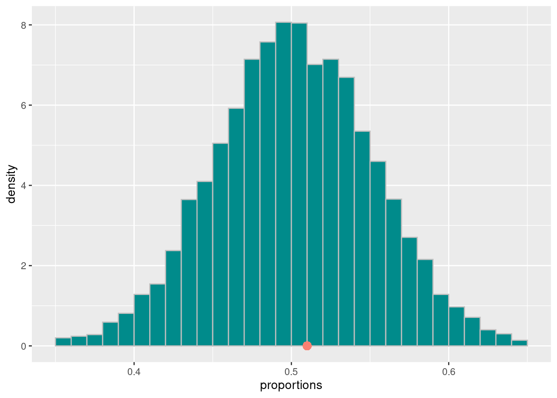

We see that the histogram looks symmetric and centered around 0.51 (see the orange dot), as expected. Neat!

4.6 Exercises

Be sure to install and load the following packages into your R environment before beginning this exercise set.

library(tidyverse)
library(edsdata)
library(gapminder)

Question 1. Every day Alana, an amateur transcendentalist and photographer, walks by a pond for one hour, rain or shine. During the walk she sometimes sees some animals. Notable ones among them: jumping fish, great blue heron, and squirrels. Over the past 80 days she has witnessed these 40 times, 40 times, and 40 times, respectively.

Question 1.1 What are the probabilities that she witnesses jumping fish, that she witnesses a blue heron, and that she witnesses a squirrel on any particular day individually? Write down three expressions that provide these probabilities and assign them to names wit_fish, wit_heron, and wit_squirrel respectively.

Alana is suspect that when she observes a jumping fish on a given day, she is more likely to also encounter the other two animals on the same day. Likewise if she first sees a great blue heron or a squirrel.

The tibble alana from the edsdata package is the actual record of Alana’s witnessing events.
```
alana
```
```
## # A tibble: 80 × 4
##      day heron  fish squirrel
##    <int> <dbl> <dbl>    <dbl>
##  1     1     0     0        0
##  2     2     0     0        0
##  3     3     1     1        1
##  4     4     1     1        1
##  5     5     1     1        1
##  6     6     0     0        0
##  7     7     0     0        0
##  8     8     0     1        1
##  9     9     1     1        1
## 10    10     1     1        1
## # … with 70 more rows
```
The rows are the 80 days and the columns are witness (1) or non-witness (0) of the three animals.
Question 1.2 If the observational unit is an individual observation made by Alana during her walk, then the tidy data guidelines tell us that each row contains multiple observations. Let us tidy the alana tibble using a tidyr function so that the three variables become materialized: day, animal_observed, and witness. Call the resulting tibble alana_tidy.
Question 1.3 Form a tibble called summarized_observations that gives the total number of times that Alana saw each of the three animals during her trip (or, more technically, the total number of 1 witnessing events for each animal). The tibble should have two variables named animal_observed and n. Do the values match the stated counts of 40?
Question 1.4 From your tibble alana_tidy, extract the number of days in which Alana witnessed all three animals. Store your answer (a single double value) in the name observed_witness3.

Question 2 We can now apply simulation to help address Alana’s question. That is, we will assume that the true probability of observing any of the three animals follows what you found in Question 1 and that the observation of one animal has no influence on the observation of any of the other two animals (i.e., each observation is independent of the other).

We can then simulate Alana’s 80-day trip a great number of times. More specifically, we will simulate the number of days Alana saw all three animals during the said “artificial” trip. If the actual record of observing all three animals is different from what our simulation shows, we have evidence that supports Alana’s claim that the probability of observing some animal may be dependent on the probability of first observing any of the other two. That would be welcome news – no more waiting around for the great blue heron!

Let us approach this simulation in parts, using the same recipe for simulation we learned. Be sure you have read and understood the examples from the textbook before proceeding.

Question 2.1 Write a function findings_from_one_walk that takes a double day as an argument and returns a tibble giving the results after one simulated walk in Alana’s trip. Here is what this tibble looks like after one possible run for day 5.

day animal_observed witness

5 heron 1

5 fish 0

5 squirrel 1

NOTE: The values in the witness column should be different every time this function is called! How to generate these values? See the sample function we saw in class.
```
findings_from_one_walk(5) # an example call for a simulated "day 5"
```
Using your function findings_from_one_walk, we can simulate a full 80-day trip as follows:
```
map(1:80, findings_from_one_walk) |>
  bind_rows()
```
Question 2.2 Write a function one_alana_trial that takes no arguments, simulates a full 80-day trip, and returns the number of days that all three animals were witnessed. The result should vary each time it is run.

HINT: To complete this, you can re-use code you have already written, i.e., from Question 4 in Part I.
```
one_alana_trial() # an example call
```
The returned value from your function one_alana_trial() composes one simulated value in our simulation.
Question 2.3 We are now ready to put everything together and run the simulation. Set a name num_repetitions to 1,000. Run your function one_alana_trial() num_repetitions number of times and store the simulated values in a vector named witness3_trials.

NOTE: This may take a few seconds to run.
Question 2.4 Construct a tibble named results by aligning num_repetitions (create a sequence from 1 to num_repetitions) and witness3_trials with the column names repetition and witness3_trial, respectively.
Question 2.5 Using ggplot2, generate a histogram of witness3_trial from the tibble results. Remember to plot in density scale; you may also wish to lower the number of bins to a smaller value, say, 10. Your plots should label all axes appropriately and include a title informing what is being visualized.
Question 2.6 Compare your histogram with the value observed_witness3 computed earlier. Where does it fall in this histogram? Is it close to the center where the “bulk” of the simulated values are?
```
observed_witness3
```
Question 2.7 Based on what you see in the above histogram and how it compares with observed_witness3, what would you say to the following statement: “since each animal is observed 40 out of 80, the chance of seeing all three animals after first seeing one of them is still 50-50, about the same as the chance of heads or tails after a fair coin toss”?

day	animal_observed	witness
5	heron	1
5	fish	0
5	squirrel	1

Question 3. A friend recently gave Cathy a replica dollar-coin. Cathy noticed that the coin has a slight bias towards “Heads”. She tossed it a few times to find that the Heads/Tails ratio is like 3 to 2; that is, if she tosses the coin five times, she would observe three Heads and two Tails among the five outcomes. Noticing the curious behavior, Cathy asked a friend Jodie to play the following game with her. For preparation, Cathy and Jodie each prepare a pile of ten lollipops. Then they would repeat the following ten times.

Jodie predicts Heads or Tails and Cathy tosses the coin. If the prediction matches the outcome, Jodie takes one lollipop from Cathy’s pile; if the prediction does not match the outcome, Cathy takes one lollipop from Jodie’s pile.

Let us do some analysis of the game.

Question 3.1 We have collected the results from one round of the game in the vectors jodie_predictions and outcomes. How many lollipops does Jodie have now?

jodie_predictions <- c("Tails", "Tails", "Heads", 
                       "Heads", "Tails", "Tails", 
                       "Heads", "Tails", "Tails", 
                       "Heads")
outcomes          <- c("Tails", "Heads", "Heads", 
                       "Heads", "Heads", "Tails", 
                       "Heads", "Heads", "Heads", 
                       "Tails")

Question 3.2 Suppose Jodie selects either side of the coin with equal chance, i.e., she does not favor “Heads” anymore than she does “Tails” and vice versa. Based on the observation that Cathy’s coin follows a “Heads”/“Tails” ratio of 3:2, after one round of the game how many lollipops is Jodie expected to lose to Cathy?

Let us use simulation to check our analysis of the problem. We will define two functions, simulate_cathy_coin() and simulate_jodie_prediction(), that simulates a single flip of Cathy’s coin and Jodie’s prediction of the side a coin lands on, respectively.
```
simulate_jodie_prediction <- function() {
  # Jodie chooses either side of a coin with equal chance. 
  sample(c("Heads", "Tails"), prob = c(1/2, 1/2), size = 1)
}
simulate_cathy_coin <- function() {
  # Cathy's coin is known to be biased towards "Heads" in a 3:2 ratio. 
  sample(c("Heads", "Tails"), prob = c(3/5, 2/5), size = 1)
}
```
Question 3.3 Write a function called one_flip_lollipop_wins that simulates the number of lollipops Jodie wins after one flip of Cathy’s coin. The function receives two arguments, a prediction function coin_flip_func and a coin flip function prediction_func; these should be called in the duration of the function to simulate a flip of Cathy’s coin and Jodie’s prediction of that coin. The function returns either 1 or -1. We can interpret 1 to be Jodie winning one lollipop and -1 to be Jodie losing one lollipop.
```
# An example call using the functions corresponding 
# to the game Cathy and Jodie are playing. 
one_flip_lollipop_wins(simulate_cathy_coin, simulate_jodie_prediction)
```
Question 3.4 One round of the game Cathy and Jodie are playing consists of 10 coin flips. Write a function named gains_after_one_round() that simulates the number of lollipops Jodie wins after one round of the game. The function receives three arguments, flips, the number of flips in a round, coin_flip_func, and prediction_func. The function returns the number of lollipops Jodie wins after the round is over. Use the replicate construct to call one_flip_lollipop_wins() a number of times.
```
# One round consists of 10 coin flips. 
gains_after_one_round(10, simulate_cathy_coin, 
                      simulate_jodie_prediction)
```

Question 3.5 Let us now simulate the game a large number of times. Using the replicate construct with the function gains_after_one_round(), simulate 10,000 games. Collect the lollipops won from each simulated game in a vector named simulated_gains.

The following function hist_from_simulation() produces a histogram of the simulated gains you generated.

hist_from_simulation <- function(simulated_results) {
  wins_tibble <- tibble(
    repetition = 1:length(simulated_results),
    gain = simulated_results
  )

  g <- ggplot(wins_tibble) +
    geom_histogram(aes(x = gain, y = after_stat(density)),
                   bins=12,
                   color = "gray", fill = "darkcyan")
  return(g)
}

hist_from_simulation(simulated_gains)

Question 3.6 What value does the bulk of the data center around? Does this agree with or contradict our earlier analysis in Question 3.2?
Question 3.7 Cathy proposes to switch roles. In other words, Jodie will toss the coin, and Cathy will predict. Knowing about the bias of her coin, Cathy bets on predicting “Tails” every time. Write a function simulate_cathy_prediction that receives no arguments and simulates Cathy’s prediction under this scheme.
Question 3.8 Repeat Question 3.5 but now using simulate_cathy_prediction(). Assign your simulated values to the name simulated_gains_switched_roles. Then generate a histogram of the results using hist_from_simulation().
Question 3.9 Where is the bulk of the data centered around now? Is the prior knowledge of the coin’s bias helpful for winning more lollipops in the long run? Or does Cathy come out the same regardless of who is making the predictions? Explain your reasoning.
Question 3.10 It will be helpful to visualize the two histograms in the same plot. Using simulated_gains and simulated_gains_switched_roles, generate an overlaid histogram showing the simulated results when Jodie predicts the coin flip together with the results when Cathy predicts the coin flip. Your plot should include a legend showing which histogram corresponds to which player making the predictions.

HINT: Before writing any ggplot2 code, you will need to develop a tibble that contains the results from both. See the code in hist_from_simulation() for some hints on how to accomplish this.

Question 4 This question is a continuation of Question 3.

Suppose we make a further change to the rule of the game so that the game will continue until either player loses all their lollipops. If one round is defined as a single coin toss, how many rounds will it take for them to complete the game? Let us compute the number of rounds by simulation.

Suppose that Jodie and Cathy each begin with 10 lollipops in their pile. There are two different ways the game ends.

One is by Jodie losing all her lollipops,
The other is by Cathy losing all her lollipops.

We have seen that the present strategy (Cathy always predicts “Tails”) slightly favors Cathy winning. The histogram that follows this strategy clusters around a small negative value, approximately -2. We thus use a positive round number if Jodie loses the lollipops and the round number with the sign flipped if Cathy loses the lollipops.

We can accomplish the simulation scheme using the incantation:

gains_after_one_round(1, simulate_cathy_coin, simulate_cathy_prediction)

We can then use the accumulate construct shown in Sections 6.3 and 6.4. Recall that we can use this to call some function repeatedly, each time using the result of the previous application as the argument.

Question 4.1 First, write a function total_lollipops_after_play that takes a single argument jodie_lollipops that gives the current number of lollipops in Jodie’s pile. This function:
- Checks if Jodie lost all her lollipops (Jodie’s pile contains 0 lollipops) or Cathy lost all her lollipops (Jodie’s pile contains 20 lollipops). If this condition succeeds, the game should be terminated by calling done() in a return call, i.e., return(done())
- Otherwise, simulate one round of the game as shown above. Save the result to a name gains. The function returns the addition of gains and the argument lollipops.
```
total_lollipops_after_play <- function(jodie_lollipops) {

}
```
Question 4.2 Write another function play_until_empty_pile that takes no arguments. This function will:
- Simulate total_lollipops_after_play using the accumulate function. Call accumulate for a maximum of 1,000 rounds (e.g., using the input sequence 1:1000) using the number of lollipops Jodie starts with as the initial value.
- Determine how many lollipops remain in Jodie’s pile after the game is over. This can be done by inspecting the last value in the vector returned by accumulate. Call this num_remaining.
- If Jodie lost (how can you tell?), the function returns the number of rounds played.
- Otherwise, if Jodie won (how can you tell?), then the functions the negative of the round number.
```
play_until_empty_pile <- function() {

}
```
The following is an example call of your function. The total number of rounds played will be different each time the function is called. Most of the time you will observe a positive value.
```
play_until_empty_pile()
```
Question 4.3 Simulate the game 10,000 times and collect the results into a vector named simulated_durations.
Question 4.4 What are the maximum and the minimum of simulated_durations? How about the mean? According to these results, who is the winner in the long run? Is it true that Cathy always wins when she predicts “Tails”?
Question 4.5 Plot a histogram of the simulated duration values. Set the number of bins equal to 25.
Question 4.6 What does the shape of the distribution you found tell you about who wins in the long run? Can this histogram be used to draw such a conclusion?

Question 5: The Paradox of the Chevalier De Méré French people used to love (maybe still do) gambling with dice. In the 17th century, Antoine Gombaud Chevalier De Méré stated that the following two events are equally probable.

throwing a dice four times in a row and 1 turning up at least once, and
throwing a pair of dice 24 times in a row and two 1’s simultaneously turning up at least once.

His logic was as follows:

There are six faces to a dice. The chance of observing the first event is $4*(1/6) = 2/3$ because there is a $1/6$ probability of a 1 turning up on a single roll and the dice is rolled 4 times.
There are six faces to each dice. The chance of observing the second event is $24*(1/36) = 2/3$ because there is a $1/36$ probability of two 1’s turning up after a single roll and the pair is rolled 24 times.
Unfortunately, there is a flaw in his logic. Using a bit of probability analysis, we have:
There are six faces to a dice, so the chances of observing the first event is the opposite of seeing anything but 1 four times in a row, which is $1 - (5^4 / 6^4) = 0.517746...$.
There are 35 outcomes that are not a double 1’s when rolling a pair of dice (out of 36 possible). Thus, the chance of observing the second event is the opposite of seeing any of those 35 outcomes 24 times. So we have: $1 - (35^24/36^24) = 0.491403...$.

Not only the two values are different from each other, but also they are different from $2/3$.

We are lucky that the theoretical analysis here has been straightforward. That is because we are able to take advantage of the fact that the events “at least one 1 turns up” and “no 1s turns up” are complementary. This is also sometimes called the “rule of subtraction” or the “1 minus rule”.

However, theoretical analysis can be cumbersome and, depending on the problem, is not always possible. Sometimes it is easier to find the answer using simulation! Let us try to disprove the Chevalier’s estimation by means of simulation.

Following is a function simulate_dice_roll that simulates one dice roll:

simulate_dice_roll <- function() {
  sample(1:6, size = 1)
}
simulate_dice_roll()

Question 5.1 Write a function has_one_appeared that simulates whether a 1 appears after a six-sided dice roll. The function takes no arguments and returns TRUE if the simulated roll turns up 1 and FALSE otherwise.
```
has_one_appeared() # an example call 
```
Question 5.2 Write another function called has_double_ones_appeared that simulates whether two 1s appear after rolling a pair of six-sided dice. The function takes no arguments and returns TRUE if double 1s turn up after the simulated rolls and FALSE otherwise.
```
has_double_ones_appeared() # an example call
```
Question 5.3 Write a function chavalier_first_event that simulates the Chavalier’s first event. The function takes no arguments. It should execute has_one_appeared four times and return a Boolean indicating whether a 1 has appeared.
```
chavalier_first_event() # example call
```
Question 5.4 Write a function chavalier_second_event that simulates the Chavalier’s second event. This function takes no arguments. It should execute has_double_ones_appeared 24 times and return a Boolean indicating whether a pair of dice both turned up 1.
Question 5.5 Simulate each of the Chavalier’s two events 10,000 times. Store the resulting values from each of the simulations into two vectors named simulated_values_first_event and simulated_values_second_event, respectively.

The following code chunk puts together your results into a tibble named sim_results.
```
sim_results <- tibble(
  first_event = simulated_values_first_event, 
  second_event = simulated_values_second_event)
sim_results
```
Question 5.6 Tidy the tibble sim_results using a tidyr function so that each observation in the tibble refers to the outcome of a single simulation and materializes two variables: event (referring to either the first or second event) and outcome (the outcome of that event). The resulting tibble should contain 20,000 observations. Assign this tibble to the name sim_results_tidy.
Question 5.7 Generate a bar chart using sim_results_tidy. Fill your bars according to the event in the variable event. We recommend using the “dodge” positional adjustment so that comparisons are easier to make.

Repeat Question 5.5 through Question 5.7 to observe differences in the resulting histogram, if any. Then proceed to the following question:
Question 5.8 A fellow classmate claims that the above simulation is unable to disprove the Chavalier’s flawed reasoning. He cites two reasons for his claim:
- The “first event” and “second event” bars are too close to each other to say anything with confidence.
- Because we repeated the simulation a large number of times, there is too much variability in the results.
Which of his reasons, if any, are valid? Explain your reasoning.

3 Data Visualization

5 Sampling